Dielectric Permittivity

Dielectric permittivity (\(\varepsilon\)) represents an important diagnostic physical property for ground-penetrating radar. This physical property impacts the attenuation, wavelength and velocity of electromagnetic waves as they propagate through a material. Dielectric permittivity is defined as the ratio between the electric field (\(\vec E\)) within a material and the corresponding electric displacement (\(\vec D\)):

\[\vec D = \varepsilon \vec E\]

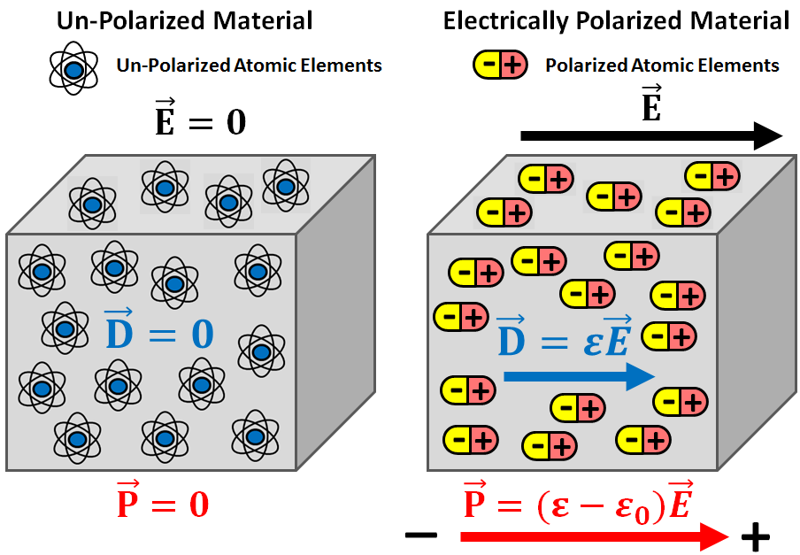
When exposed to an electric field, positive and negative charges within individual atoms and molecules try to separate from one another. For example, the electron clouds of atoms will shift in position relative to their nuclei. The extent of electrical charge separation within a material is represented by the electric polarization (\(\vec P\)). The electric field, electric displacement and electric polarization are related by the following expression:

\[\vec D = \varepsilon_0 \vec E + \vec P\]

where the permittivity of free-space (\(\varepsilon_0 = 8.8541878176 \times 10^{-12}\) F/m) defines the relationship between \(\vec D\) and \(\vec E\) if the material is non-polarizable. Therefore, the dielectric permittivity and the electric displacement define how strongly a material becomes electrically polarized under the influence of an electric field. The electrical polarization within the material can be defined in terms of the electric field as follows:

\[\vec P = (\varepsilon - \varepsilon_0 ) \vec E = \chi_e \varepsilon_0 \vec E\]

where \(\chi_e\) is known as the electric susceptibility. The electric susceptibility should not be confused with the magnetic susceptibility, as they describe different physical processes.

Relative Permittivity: The dielectric properties of materials are generally expressed using the relative permittivity (\(\varepsilon_r\)). The relative permittivity defines the dielectric properties of a material relative to that of free-space:

\[\varepsilon_r = \frac{\varepsilon}{\varepsilon_0}\]

Parameters used to define the dielectric properties of materials and their associated units are tabulated below.

Property	Symbol	Units
Electric Field	\(\vec E\)	N/C or V/m
Displacement Current	\(\vec D\)	A/m \(\!^2\)
Electric Polarization	\(\vec P\)	A/m \(\!^2\)
Dielectric Permittivity	\(\varepsilon\)	F/m
Electric Susceptibility	\(\chi_e\)	Unitless
Relative Permittivity	\(\varepsilon_r\)	Unitless

Measurements for Dielectric Permittivity

There are a host of methods for measuring the dielectric permittivity of a material. Here, we will describe two basic experiments. These experiments assume that 1) the sample is non-magnetic (i.e. \(\mu = \mu_0\)) and 2) the conductivity of the sample is sufficiently small (\(\sigma < 0.01\)).

Transmission Time Measurements

The speed at which high-frequency electromagnetic (EM) waves move through a material depends on the material’s dielectric permittivity. Assuming the material is non-magnetic, this relationship is given by:

\[v = \frac{c}{\sqrt{\varepsilon_r}}\]

where \(\varepsilon_r\) is the relative permittivity and \(c = 2.998 \times 10^8\) m/s is the speed light constant. In free-space, \(\varepsilon_r = 1\) and EM waves travel at the speed of light. However, within a dielectric material, EM waves propagate more slowly according to the above relationship.

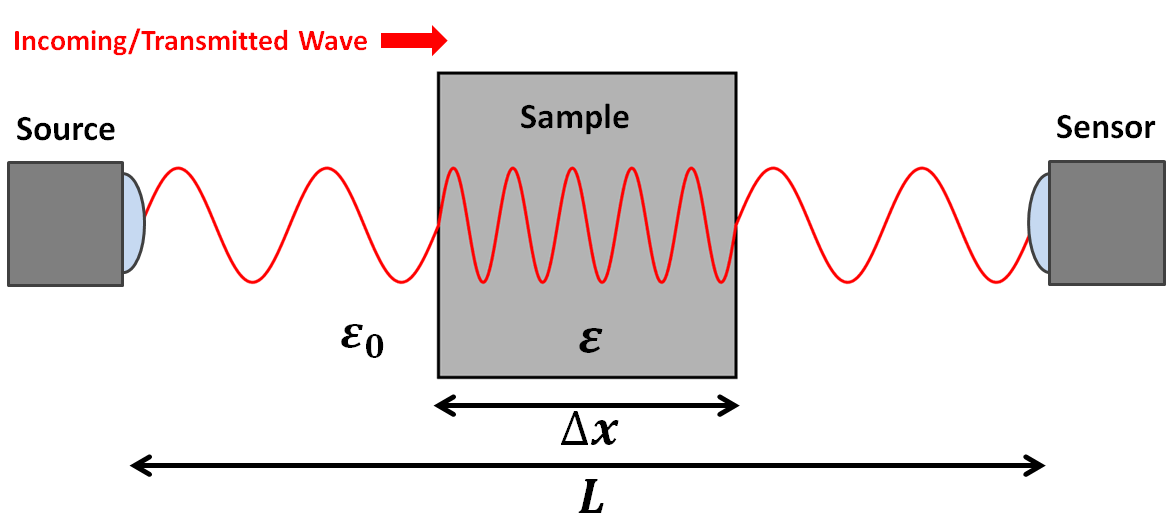
When performing physical property measurements, a source sends EM waves towards a sample. A portion of these waves transmit through the sample and reach a sensor on the other side. For samples that have high dielectric permittivities, it will take much longer for the signal to arrive at the sensor. This is because the transmitted waves slow down as they propagates through the sample. An equation for the total travel time (\(\Delta t\)) for transmitted EM waves as the go from the source to the receiver is given by:

\[\Delta t = \frac{L - \Delta x}{c} + \frac{\Delta x}{v}\]

where \(L\) is the distance from the source to the receiver, \(\Delta x\) is the length of the sample, \(c\) is the speed of light and \(v\) is the velocity of the waves as they propagate through the material. Using the signal measured by the receiver, we can determine the total travel time for the transmitted EM waves. By combining the previous two equations and solving for the relative permittivity:

\[\varepsilon_r = \Bigg ( 1 + \frac{c\Delta t - L}{\Delta x} \Bigg )^2\]

Reflection Coefficient Measurements

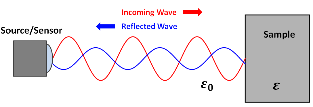
When EM waves meet an interface, some of their energy is reflected and some of their energy is transmitted. For high-frequency EM waves, the proportion of energy which is reflected depends on the dielectric properties of the materials comprising the interface. This relationship is generally characterized by a reflection coefficient. The reflection coefficient \(R\) defines the ratio between the amplitude of the reflected wave and the amplitude of the incoming wave:

\[R = \frac{A_{ref}}{A_{inc}}\]

Below is a diagram for a simplified experiment. In this experiment, a source generates EM waves which are reflected due to a difference in dielectric permittivity. The reflected waves are measured by a sensor. Assuming the incoming waves have a zero incidence angle relative to the interface, the reflection coefficient is given by:

\[R = \frac{1 - \sqrt{\varepsilon_r}}{1 + \sqrt{\varepsilon_r}}\]

where \(\varepsilon_r\) is the relative permittivity of the sample. From the source, it is trivial to determine the amplitude of incident EM waves at the interface. Using the sensor, we may also determine the amplitude of reflected EM waves at the interface. If both amplitudes are known, the first equation may be used to determine the reflection coefficient. Once obtained, the second equation may be used to solve for the relative permittivity of the sample.

Electrical Permittivity for Common Rocks

A table containing the relative permittivities for common rocks, soils and other materials is shown below (Martinez and Byrnes, 2001). Rocks within a certain classification vary significantly in composition. As a result, the relative permittivities of rock types are given as a range of values. By examining this table, several things can be inferred:

• Water has a much higher dielectric permittivity than rock forming minerals.

• Water saturated rocks have larger dielectric permittivities than dry rocks.

• Saturated sediments generally have larger dielectric permittivities than hard rocks.

• The variation in dielectric permittivity for sediments is larger than it is for hard rocks.

Material		\(\varepsilon_r\;\)
Air		1
Fresh Water		80
Sea Water		80
Ice, Snow, Permafrost
Sediments
Rocks
Minerals

Factors Impacting Electric Permittivity

Porosity and Water Saturation:

By far the most important factors in determining a rock’s dielectric permittivity are porosity and water saturation. Air has a relative permittivity of 1 whereas common rock forming minerals have much higher relative permittivities. This means that for dry samples, the rock’s bulk dielectric permittivity decreases as the porosity increases.

When rock samples are saturated with water, their dielectric permittivities can increase drastically. This is because water has a relative permittivity of 80, which is much higher than the relative permittivities of rock forming minerals. As a result, the bulk dielectric permittivity of a rock increases as pore water saturation increases.

The relationship between a rock’s bulk dielectric permittivity, porosity and water saturation is given by:

\[\sqrt{\varepsilon} = (1 - \phi ) \sqrt{\varepsilon_m} + \phi \big [ S_w \sqrt{\varepsilon_w} + (1-S_w) \sqrt{\varepsilon_a} \big ]\]

where

• \(0 \leq \phi \leq 1\) is the porosity

• \(0 \leq S_w \leq 1\) is the factional volume of the pore space saturated by water.

• \(\varepsilon_m\) is the dielectric permittivity of rock forming minerals.

• \(\varepsilon_a\) is the dielectric permittivity of air (equal to free-space).

• \(\varepsilon_w\) is the dielectric permittivity of water.

Frequency:

For hard rocks and unsaturated sedimentary samples, the dielectric permittivity can be considered constant for all intents and purposes. At sufficiently low frequencies, the same can be said about water-saturated sedimentary rocks and soils (Kaatze, 1989; Meissner and Wentz, 2004). At high frequencies however ( > 1 GHz), the electric polarization within water-saturated samples depends on the frequency of the electric field. As a result, these samples are sometimes characterized using a frequency-dependent dielectric permittivity:

\[\varepsilon (\omega) = \varepsilon^\prime (\omega) + i \varepsilon^{\prime\prime} (\omega)\]

where \(i = \sqrt{-1}\). The real component of the dielectric permittivity (\(\varepsilon^\prime\)) represents energy stored through electrical polarization whereas the imaginary component (\(\varepsilon^{\prime\prime}\)) represents a measure of energy loss. The significance of the real and imaginary components of the dielectric permittivity will be discussed in more detail when learning about ground-penetrating radar (link).

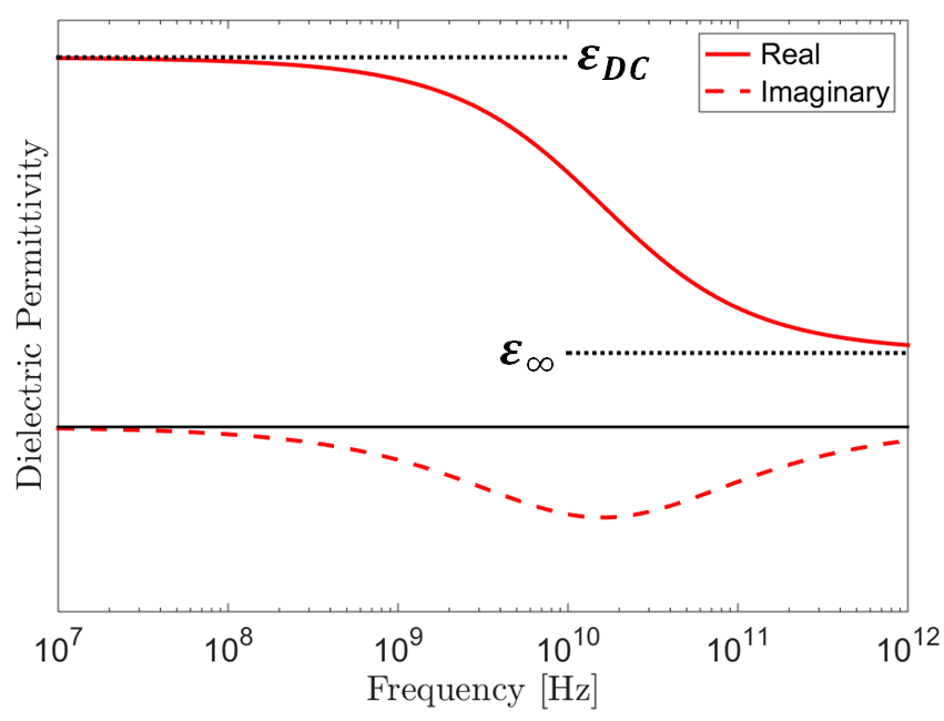
A widely used model for describing the frequency-dependent dielectric permittivity is the Cole-Cole model:

\[\varepsilon (\omega) = \varepsilon_\infty + \frac{\varepsilon_{DC} - \varepsilon_\infty}{1 + (i\omega \tau)^\alpha}\]

where \(\varepsilon_{DC}\) is the DC or zero-frequency permittivity, and \(\varepsilon_\infty\) represents a limit as frequency goes to infinity. Parameters \(\tau\) and \(\alpha\) define the span of frequencies in which the dielectric permittivity changes with respect to frequency. As we can see from this model:

• Frequency-dependence only occurs over a finite span of frequencies.

• The magnitude of the dielectric permittivity decreases with respect to an increase in frequency.

• At sufficiently low frequencies, the dielectric permittivity is constant and real-valued.