Gravity gradients
Introduction
This page is an overview of this rapidly growing aspect of gravity surveying. Important goals are to recognize what spatial derivatives are and what the total horizontal derivative is good for, understand the idea behind “second spatial derivatives,” and recognize that direct measurement of all vectoral components of the spatial gradients of both gravity and magnetics is the latest really new capability in the geophysics industry. Is it useful? Much money has been spent on inventing this capability and yes, it is useful for larger scale problems associated with oil and gas and to some extent minerals exploration.
Measured gravity is \(g_z\)
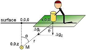
Normally the vertical component of gravity \(g_z\) is measured. This was illustrated using the profile over a sphere or cylinder (right) in the section Gravity measurements. The horizontal components of gravity, \(g_x\), and \(g_y\), are small and not measured.
The spatial derivative (rate of change) of \(g\)
The spatial rate of change of gravity (in the x-direction) is written mathematically as \(\partial g/ \partial x\). This horizontal derivative can help map edges of buried changes in density. However, when data were gathered over an area, it is more common to employ the so called total horizontal derivative, which is the square root of the sum of squared x- and y- horizontal derivatives. This is a conceptually simple idea, but challenging to actually calculate if data are not on a survey grid that is uniform. Its result is illustrated in the following figures:
Fig. 193 Bouguer gravity, contour map plotted using “shading.”
Fig. 194 Total horizontal derivative of the adjacent gravity
One way to think of spatial derivatives is to simply look at the change in “value” between adjacent stations. Another better approach for real data is to look at slopes over several stations. A least squares fit to data at several stations will yield a slope. The magnitude of this slope is a horizontal derivative. This can be done along a profile (line survey) or using a matrix of points on a map. For maps, the horizontal derivative at one location is then simply the magnitude of the slope of a plane found by least squares fit to a set of points surrounding that location.
The second spatial derivative
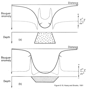
The rate of change of gradients (written as \(\partial^2 g / \partial x^2\) also can be estimated. Inflection points on the graph of \(\partial^2 g / \partial x^2\) reveal the location of maximum rate of change of the gradient. The adjacent images show how this can help reveal the difference between a basin and an intrusion. Maps can also be processed to generate images of the second horizontal derivatives.
The second vertical derivative is often considered useful. But what is the first vertical derivative? It is the vertical rate of change of gravity, and it is not easy to find unless you measure gravity everywhere at two elevations. However, gravity (a potential field) follows Laplace’s equation, which states that squared gradient of gravity equals 0:
The \(\partial^2 g / \partial x^2\) and \(\partial^2 g / \partial y^2\) terms can be obtained directly from a Bouguer anomaly map, so the \(\partial^2 g / \partial z^2\) term can be derived. This last term describes how fast the “vertical rate of change in gravity” is changing. However the success of this process depends upon adequate data spacing. These types of calculations are very efficient in the Fourier domain - something beyond the scope of this presentation.
Making these types of processed maps is sometimes useful, but not always worthwhile. Two examples are given below: 1) salt domes where the process was beneficial, 2) a mineral exploration setting where it was not so useful.
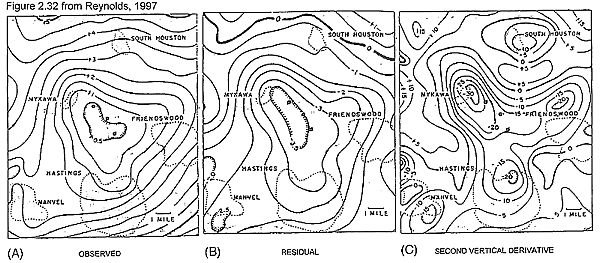
Fig. 195 Observed, residual after removing a regional component, and second vertical derivative calculated using horizontal derivatives measured from the data set. Details about the salt domes are clearer in the second vertical derivative map.
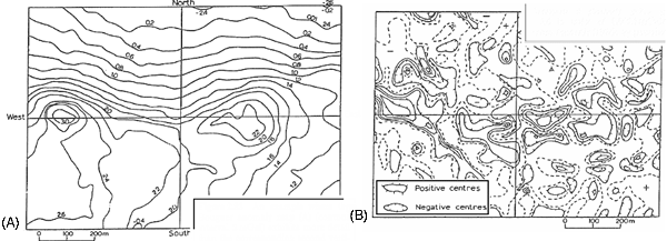
Fig. 196 The Bouguer anomaly map (A) exhibits more useful information than the corresponding second vertical derivative map (B).
An example
One recommended short example describes contributions of gravity to hydrocarbon exploration in the complicated foothills environment, just southwest of Calgary, Alberta. The take home message from that example is that sparse data forces less-than-optimal results. Gravity has always suffered from this problem (fewer measurements than desirable) because of the care required for gravity, location and elevation measurements at each station. With the invention of airborne gravity surveys, this problem can be reduced, so long as the lower sensitivity of airborne measurements is sufficient for the task. Currently airborne surveys are sensitive enough for most oil and gas exploration problems, and for some large mineral exploration problems, but not sensitive enough for engineeri & environmentalng scale work. If you are interested (it is short and easy) see Turner Valley , Canada – A Case History in Contemporary Airborne Gravity (links to the Sander Geophysics Limited (SGL) website), by J.W. Peirce1, S. Sander2, R.A. Charters1, and V. Lavoie, presented at the EAGE 64th Conference & Exhibition — Florence, Italy, 27 - 30 May 2002.
Measuring gradients
We are talking now about measuring how gravity varies spatially - that is \(\partial g / \partial x\) or \(\partial g / \partial y\) or \(\partial g / \partial z\). In fact, there are units for gravitational gradient - the Eotvos Unit (EU) which is \(10^{-6}\) mGal/cm.
However, if you think about it, we should really be more careful about what we are measuring. We are familiar with measuring the vertical component of gravity, \(g_z\). However, it would be theoretically possible to measure \(g_x\) and \(g_y\). In fact, one could consider how each of these three components of gravity vary in all three directions. That represents nine different “gradient” measurements. Given what you know about measuring \(g_z\), measuring the other two components should sound like a very difficult task. Well, you are right. It is very difficult. In fact, it turns out to be easier to measure the gradients than the fields themselves. And, as of roughly 1998 - 2001, there are systems that can make these measurements. Are they useful measurements? Yes. Oil and mineral exploration companies would not have spent millions of dollars developing the capacity if it were not useful. But there is much research needed to learn how best to make use of the results.
Maps showing what measurements of gravitational gradients look like are given on a separate page of images . Evidently, different components emphasize different aspects of a buried density contrast or target. Look at these figures and consider these questions:
Which emphasizes the feature’s location? (answer = \(T_{zz}\))
Which emphasize lineations in one or another direction? (answer = \(T_{xx}\), \(T_{yy}\))?
Which emphasize the feature’s edges? (answer = \(T_{xz}\), \(T_{yz}\))?
What does the remaining component emphasize? (answer = edges)?
Consider some practical questions: How useful is this type of work? What kinds of targets can be detected?
The answers are usually expressed in terms of anomaly size, sampling rate, and noise level of instruments.
Current systems can just see very large mineral targets.
Many oil and gas and structural geology targets can be imaged.
Anticipated limit for future systems is a little better.
Other forms of processing for maps
In the present version of this module we do not have time to include a section that pursues other aspects of deriving alternative forms of images from gravity (and magnetics) maps. It is true, however, that there are many forms of processing that are used. Two excellent introductions can be found at the following locations:
If you are interested, there are some interactive figures on frequency domain filtering at http://www.geoexplo.com/airborne_survey_workshop_filtering.html.
There is a good summary of Advanced Processing of Potential Fields by Getech (Houston, and Leeds). See the tutorial on-line at Getech via Advanced Processing of Potential Field Data.