Gravity example
Regional trend removal for gravity anomaly detection
The geophysical task
The Garber oil field in north-central Oklahoma was discovered in 1916, and has been one of the largest oil fields in the state. A gravity survey started in 1939 was terminated before completion because no anomaly could be seen with the station spacing of 805 m. The author returned to collect gravity data at 201 m spacing in 1950 in order to ascertain whether more careful work could detect the anomaly expected from the formations known to be present. Figure 1a is the resulting Bouguer anomaly map, with the profile discussed below shown as A-A’.
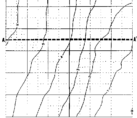
Fig. 191 Figure 1a. Bouguer gravity map of the area of interest. Contour interval is 1 mGal. l.
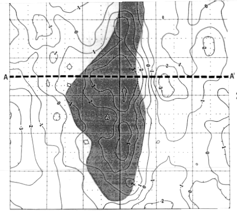
Fig. 192 Figure 1b. Residual gravity anomaly after removing third degree best fit polynomial. The gray zone is the producing area of this oil field.
Method
Three methods were employed to resolve the the local anomaly from the regional anomaly.
First, a third degree polynomial surface was fitted to the Bouguer anomaly map; then the resulting trend was subtracted from the Bouguer anomaly map. The result is shown in Figure 1b, with the oil-producing structure overlaid as a gray zone. Good correspondence between the residual anomaly and the geological structure of interest is evident.
The second trend removal technique involved calculating a vertical gradient map from the Bouguer anomaly map. Results were similarly successful at delineating the structure.
The third method involved harmonic analysis of data along the profile. Please refer to the original paper for details.
Discussion
The figure below shows the Bouguer anomaly, the polynomial regional trend, the vertical gradient, the residual after subtracting the trend from the Bouguer anomaly, and the forward modeled response to structures associated with the oil field. Several points are worth noting:
It is not surprising that the original gravity survey with spacial interval of 800 m failed to identify the target. Clearly, 200 m spacing was much more appropriate.
The anomaly associated with interesting structures is easy to miss if the regional trend is not properly removed.
Trend removal is implicit when gradient filtering is applied. Vertical gradient filtering is shown, but horizontal gradients would also likely identify the structure.
Significant fault zones are identified by high lateral gradients in both the residual and the vertical gradient profiles.
The 2D model used to calculate an expected response (using the commonly applied method of Telwani) was well understood at the time of the test. There are undoubtedly other structures that could produce similar gravitational response at the surface
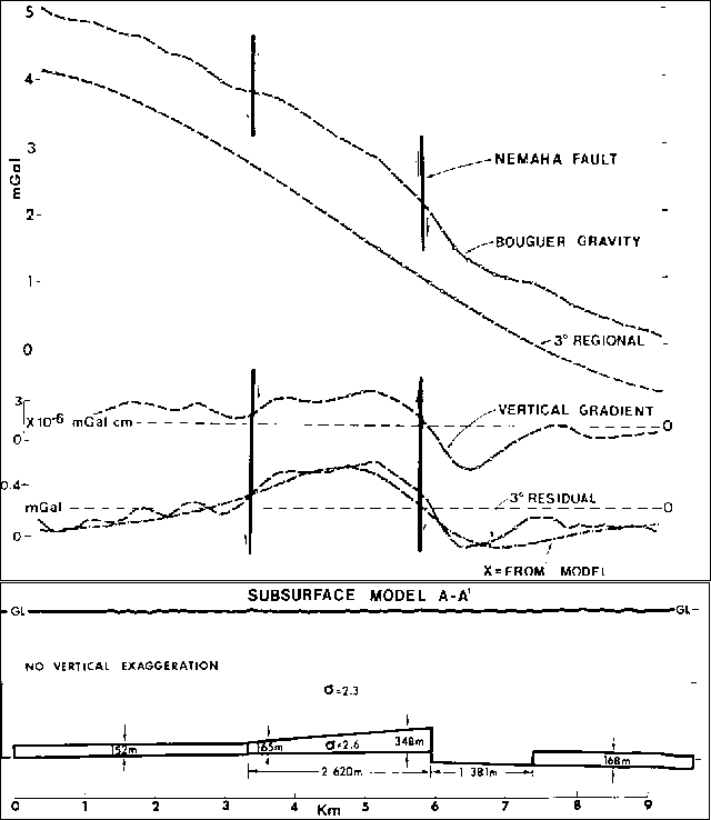
Top: Four profiles (A-A’ in Figure 1) showing (top to bottom) the Bouguer gravity anomaly, the third degree polynomial, the vertical gradient, and the residual (Bouguer anomaly minus regional). The modeled response is also shown with the residual profile.
Bottom: The model used to generate the modeled profile in the top panel. Densities and geometries are quite well known from oil well drilling that has taken place since the Garber field was discovered in 1916.
Original Reference
This example is summarized from C. Ferris, 1987, Gravity anomaly resolution at the Garber field, Geophysics, 52, #11, 1570-1579.