Normal MoveOut (NMO): Stacking Data in CMP Gathers

Imagine recording four seismic traces from one source. If we plot the travel time for a seismic signal as a function of distance between receiver and source we see that time increases (middle panel). The curve through the traces forms a hyperbola.

For horizontal flat surfaces, the change in travel time for a set of increasing source-receiver spacings of a CMP gather (bottom panel) will be identical to the “common shot gather” (top panel). The travel time curve from the reflector will appear approximately as a hyperbola. Unlike for the common shot gather, in the CMP gather all of the arrivals correspond to the same reflection point.

The hyperbolic representation for the travel time curve is exact if the velocity above the reflector is constant, and if the reflector is flat. For layered media we saw that the travel time curve was hyperbolic, but the velocity used should be the RMS velocity. Unfortunately we don’t know what this velocity is, so we attempt to estimate it from the data themselves. We proceed as follows.

1. Assume that each reflection event in a CMP gather has a travel time that corresponds to a hyperbola,

\[t^2 (x) = t_0^2 + \frac{x^2}{v_{st}^2}\]

where \(v_{st}\) is a “stacking” velocity, or sometimes called the Normal Moveout Velocity, \(v_{nmo}\).

2. For each reflection event hyperbola, perform a velocity analysis to find \(v_{st}\). This is done by first choosing \(t_0\). Then choose a trial value of velocity \(v_1\). The associated travel time hyperbola is generated and it forms a trajectory on the CMP gather. Sum the energy of the seismic traces along the trajectory and plot this value on a graph of velocity versus energy. Repeat this procedure for different trial velocities. Choose as \(v_{st}\) the velocity that yields the largest energy. In the diagram below \(v_2\) represents the stacking velocity. The term cross power can be interpreted as total energy.

Fig. 81 From Kearey, Philip and Micheal Brooks, An Introduction to Geophysical Exploration. 2nd ed. Blackwell Science: 1991.

3. Calculate the Normal Moveout Correction: Again, using the hyperbola corresponding to \(v_st\), compute the normal moveout for each trace and then adjust the reflection time by the amount \(\Delta T\).

4. Finally, stacking the normal moveout corrected traces generates a single trace. Each trace corresponds to a zero-offset trace, that is, the seismic trace that would have been recorded by a receiver that is coincident with the source.

As an example consider the two CMP gathers in the figure below left (click for a larger version). The most prominent seismic wavelet at times between 50 and 70 ms is a bedrock reflection from about 9 m below the surface. The geophone offsets were 3.7 m (12 ft) for the nearest traces and 17 m (56 ft) for the farthest trace with 1.22 m (4 ft) between geophones. The reflection even of interest is at about 55 msec.

In the figure above right, the CMP gather for point 988 has been moveout corrected using different velocities. The moveout correction using a velocity of 1225 ft/s (328 m/s) causes the reflection events to occur at about the same time for all traces. Stacking these signals will produce a high quality reflection signal. Conversely, a velocity of 1075 ft/s is too small and produces too large a correction at far offsets.

To show what happens if the wrong velocity is chosen for carrying out the normal moveout correction, five 12-fold CMP traces are shown (right) processed with three different velocities. When the velocity is too low, the frequency of the reflection wavelet is lowered and it is therefore depicted too shallow on the seismic section. When the velocity is too high the frequency decreases and the reflection wavelet is depicted at too large a time on the seismic section. The correct velocity gives the correct position for the wavelet and preserves the high frequencies which allow best resolution of small features and thin beds. Correct velocity is about 373 m/s (1225 ft/s).

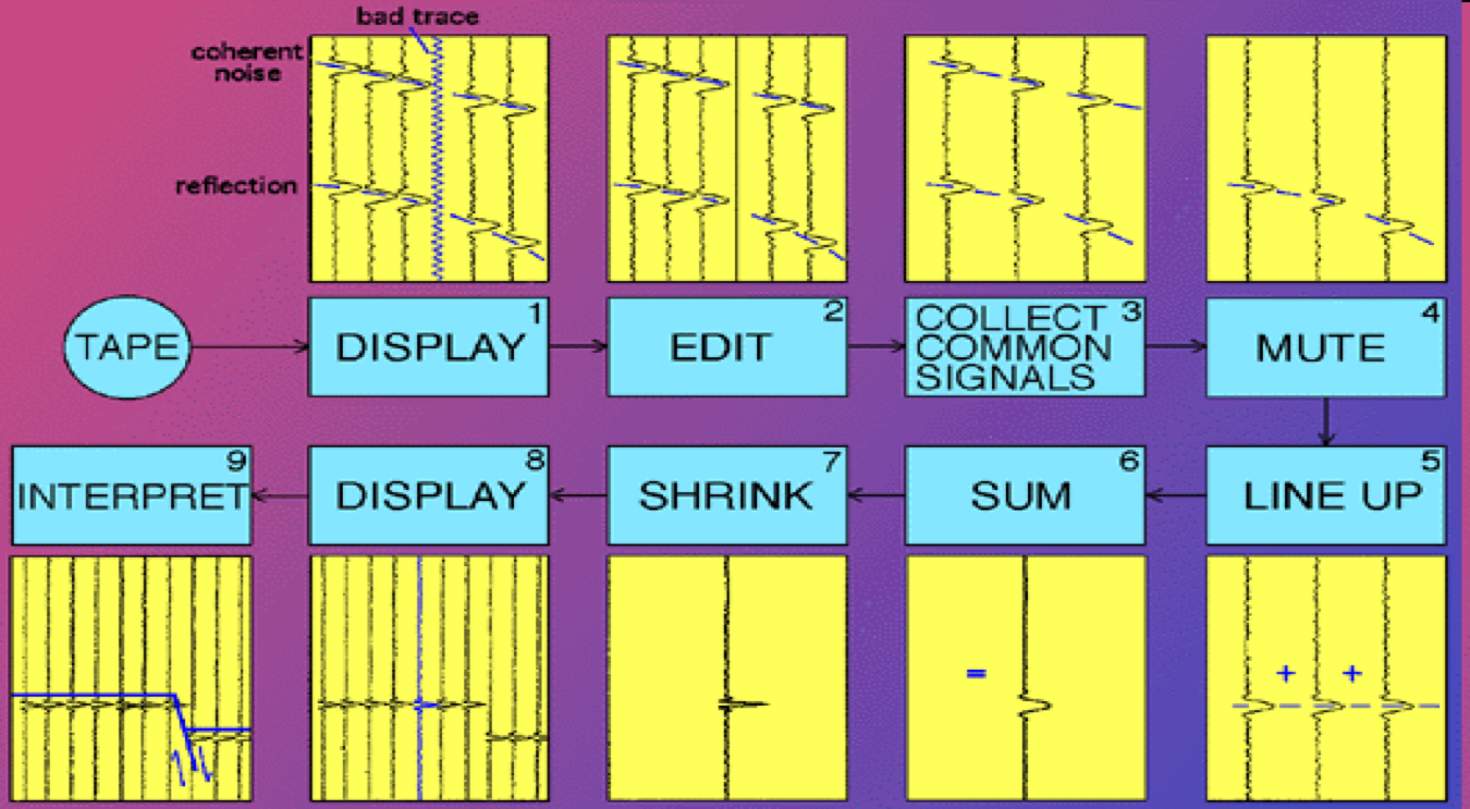
Summary: Essential Elements in CMP Processing

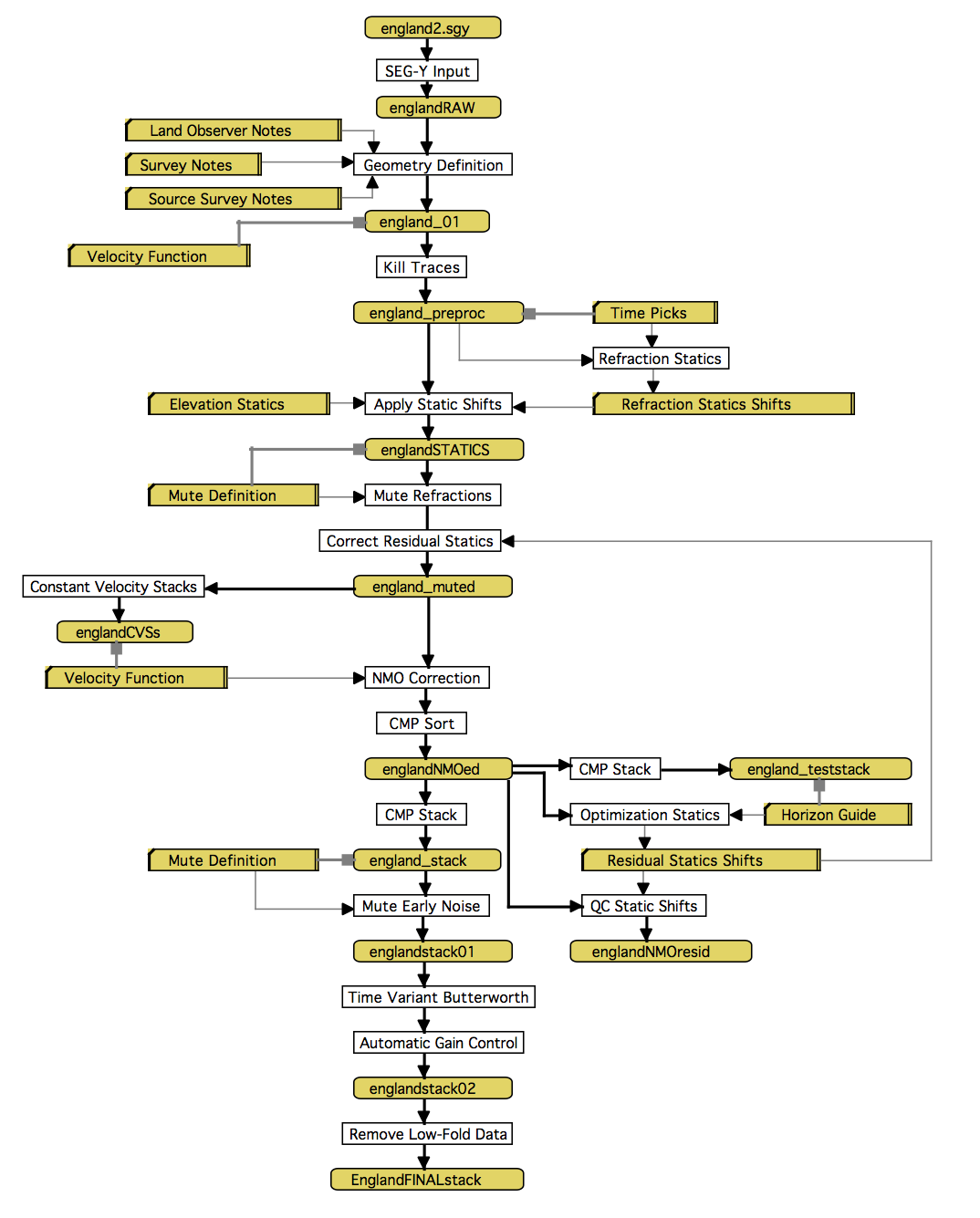
There are many different processing steps that could be performed. An example from GS Baker 1999, is shown in the flow chart image here (click for a larger version.). However, the essential steps are summarized in the following short list.

1. Obtain CSP (Common Source Point) gathers.

2. Sort into CMP (Common Midpoint) gathers. Reflection events (coming from approximately the same point in the earth) appear as hyperbolic trajectories. The goal is to stack them into a single trace.

3. For each event, perform a velocity analysis to find the stacking velocity.

4. Perform NMO correction and stack. This yields a single trace corresponding to a coincident source and receiver.

5. Composite the traces into a CMP processed section.

These are the only steps we will be concerned with in these notes. Other steps may be used by experienced contractors and they may be necessary to produce more useful sections for interpretation, but the details are beyond the scope of this set of notes.