Normal Incidence Reflection Seismogram

The principles of the normal incidence reflection seismogram are illustrated in the diagrams below. A source and receiver are at the surface of a layered earth whose properties are variable. The reflection and transmission coefficients depend upon the change in acoustic impedance, and thus on both density and velocity. The travel time for the wave to go from the source to the reflecting interface and back to the surface depends only upon the length of the travel path and the velocity of each layer. The travel time formula given below, is for a wave which travels vertically and for which the source and receiver are coincident. (The source and receiver are offset slightly in the diagram for visual clarity). This produces the “normal incidence” seismogram.

The procedure for generating the ideal seismogram is as follows:

1. Begin with a geologic section.

2. Compute the acoustic impedance as a function of depth by taking the product of the density and velocity logs

3. Compute the reflection (and transmission) coefficients as a function of depth. This yields a reflection log.

4. Convert to time. Each layer has a defined velocity. The incremental (two- way) travel time on each layer is \(\Delta t_i = 2h_i / v_i\). This yields a reflection function on the two-way travel time domain.

5. Convolve the reflectivity function with a source wavelet. This yields the desired ideal seismogram.

The figure below illustrates the procedure:

The acoustic impedance for the ith layer is given by:

\[Z_i = \rho_{i} v_{i}\]

If the amplitude of the incident ray is \(A_0\) and the amplitude of reflection is \(A_1\), then the reflection coefficient \(R\) is \(A_1/A_0\). Similarly, if the amplitude of the transmitted wave is \(A_2\), then the transmission coefficient \(T\) is \(A_2/A_0\).

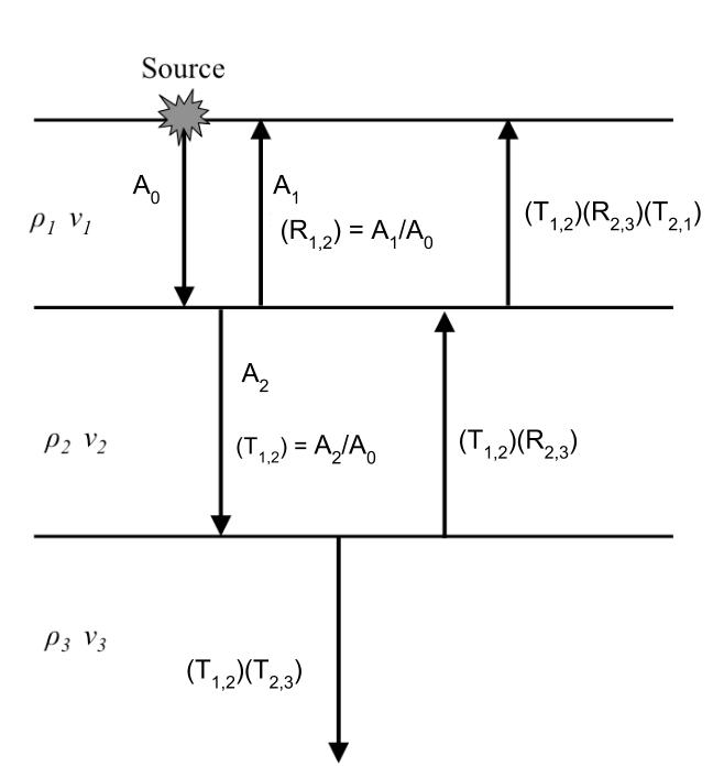
Using boundary conditions to ensure the continuity of stresses and displacements at the interface between we can express the reflection and transmission coefficients in terms of the acoustic impedance. Where \(i\) denotes the layer the wave is in and \(j\) denotes the layer that the transmitted wave passes into.

\[R_{i,j} =\frac{Z_{j} - Z_{i}}{Z_{j} + Z_{i}}\]

and

\[T_{i,j} = \frac{2Z_i}{Z_{j} + Z_{i}}\]

Given the amplitude of the incident wave \(A_0\) you can calculate the amplitude of a transmitted of reflected waves in any layer. For example, the amplitude of the transmitted wave in the 3rd layer is equal to \(A_0 T_{1,2} T_{2,3} = A_2 T_{2,3}\) and the amplitude of the reflected wave from the top of the 3rd layer in the 1st layer is \(A_0 T_{1,2} R_{2,3} T_{2,1}\).

We then convert the reflectivity log from reflectivity as a function of depth to reflectivity as a function of time. The total travel time is the sum of the incremental times for a particular reflection. The incremental 2 way travel time for layer \(i\) is:

\[\Delta t_i = \frac{2h_i}{v}\]

The normal incidence seismic trace is then obtained by the convolution of a seismic wavelet (input pulse) with the reflectivity function. The amplitude of each spike on the reflectivity function is determined by the value of the calculated reflection and transmission coefficients. The times for each reflection event are obtained by knowing the layer thickness and velocities. Each impulse on the reflection function generates a scaled replication of the seismic wavelet. The composite of all of the reflection events generates the seismic trace.

Fig. 76 The reflection seismogram viewed as the convolved output of a reflectivity function with an input pulse. 1

Notice how the negative reflection coefficients change the polarity of the signal recorded at the receiver.

Fig. 77 A synthetic seismogram. 1

1(1,2)

From Kearey, Philip and Micheal Brooks, “An Introduction to Geophysical Exploration”. 2nd ed. Blackwell Science: 1991.