Processing

So far, we have used radargrams to represent the data collected by GPR sensors. In order to create these images, some processing is required. Here, we discuss how raw GPR data are processed before they are represented using radargrams.

Travel Time to Depth Conversion

The data measured by the GPR system is the amplitude of the signal as a function of its two-way travel time. However, interpretation can be made easier if the information can be represented in terms of depth. Because of this, an apparent depth axis is frequently added to the right-hand side of the radargram.

To convert the two-way travel time to apparent depth, we must choose a propagation velocity. This may be acquired from the initial radargram, from a-priori information, or sometimes left as the speed of light (\(c = 3.00 \times 10^8\) m/s). The conversion between each vertical axis is given by:

\[d_a = \frac{V t}{2}\]

where \(d_a\) is the apparent depth, \(V\) is the propagation velocity and \(t\) is the two-way travel time. Below, we see an example where the propagation velocity is \(V = 0.13\) m/ns. From this, we can infer that the linear feature in the radargram is roughly 7-8 m away from the source and receiver.

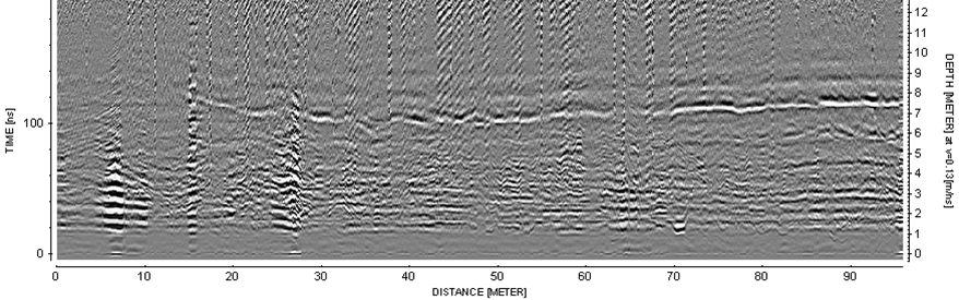
Fig. 125 Example of a radargram with apparent depth on the right axis. This assumes a propagation velocity of 0.13 m/ns.

Gain Correction

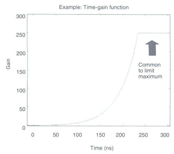
Fig. 126 Example gain function which corrects for a loss in signal strength at later times.

Signals measured at earlier times are much stronger than signals which are measured at later times. This may be due to scattering, attenuation, geometric spreading or reflection/transmission events. As a result, it may not be easy to distinguish important features in the data at later times. To account for this, the raw data \(d_{raw}(t)\) for each reading is multiplied by a gain function \(g(t)\) as follows:

\[d(t) = g(t) \times d_{raw}(t)\]

where \(d(t)\) is the data represented in the radargram. The gain function itself is a positive function which increases in magnitude as a function of time. Thus a larger gain is applied to raw data at later times. An example of the gain function is shown on the right. As we can see, the gain function increases in value exponentially to account for the exponential loss in return signal strength over time. However, the gain function is generally bounded by a maximum value.

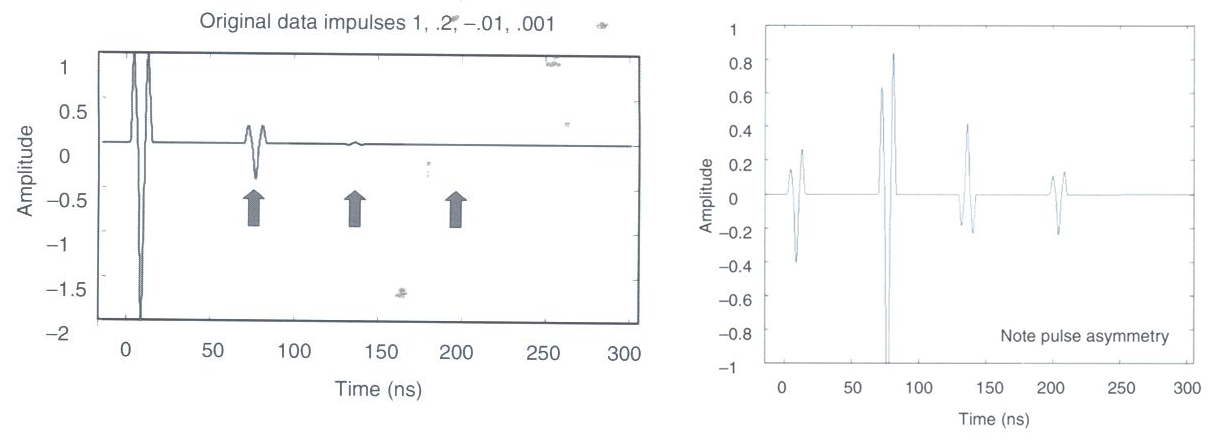
Fig. 127 (Left) Single trace before gain correction. (Right) Single trace after gain correction.

The strength of returning signals is also much weaker at distances further away from the source. Because of this, gain corrections may be applied based on Tx-Rx distance. This is not necessary for common offset surveys, but may be important in common midpoint or transillumination surveys.

Stacking

GPR signals travel at velocities close to the speed of light (c = \(3.00 \times 10^8\) m/s). As a result, the total travel times for GPR signals are on the order of 100s of nanoseconds. Because of this, it is easy to repeat the same GPR shot many times over a short interval.

Stacking describes the process of averaging a set of repeated GPR shots in order to reduce noise and improve interpretation. Essentially, stacking acts as a way of improving the signal to noise ratio for GPR data collected at a certain location. An example of this is demonstrated below. As we can see, the more readings we stack, the clearer we see coherent GPR signals.

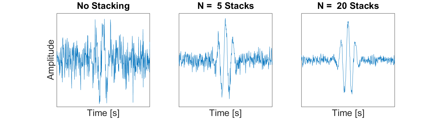
Fig. 128 Example of how averaging multiple traces from the same Tx-Rx pair can improve the signal to noise ratio. This results in an improved image of the returning signal.

Smoothing

Smoothing is another technique used to improve the interpretation of field collected GPR data. In GPR systems, the data sampling rate is such that the returning wavelet signals should be reasonably smooth and visible. Random noise on the other hand is completely incoherent. When smoothing is applied to the data, it has the effect of reducing the amplitude of incoherent noise while retaining naturally smooth signals in the data. One example of smoothing techniques is the moving average (shown below). We can see that as more data points in time are used for the average, the more easily recognizable the wavelet signal is.

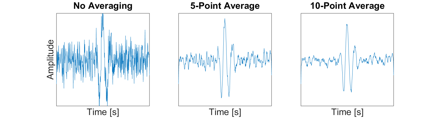
Fig. 129 Example of smoothing a trace by using a moving average.