Data

Introduction

For DC resistivity surveys, the energy source is a generator which injects a constant current into the ground using two electrodes. The “signals out” (data) are voltages measured at various places on the surface, along with strength of the known current source (in Amperes) and details about relative geometry of the four electrodes.

In order to create maps or graphs of raw data for quality assessment or for direct interpretations, measurements are converted into a form that is related to the relevant physical property. For each measurement, a 3D version of Ohm’s Law is used to generate a datum with units of resistivity (or conductivity). These transformed data are called apparent resistivities because they represent the earth’s true resistivity only if the ground is uniform. When subsurface resistivity varies, interpretation must be based upon the way in which apparent resistivity varies as a function of electrode geometry and position. The commonly used survey procedures are explained later on this page, after discussions about current flow, sources, measurements, and conversion to apparent resistivities.

Apparent resistivity

If there are two current (source) electrodes, the potential is the superposition of the effects from both. In a practical experiment (figure below), one electrode, \(A\), is the positive side of a current source, and the other electrode, \(B\), is the negative side. The current into each electrode is equal, but of opposite sign. For a practical survey, we need two electrodes to measure a potential difference. These are \(M\), the positive terminal of the voltmeter (the one closest to the \(A\) current electrode), and \(N\), the negative terminal of the voltmeter.

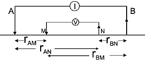
The measured voltage is a potential difference \((V_M - V_N)\) in which each potential is the superposition of the effects from both current sources:

\[\begin{split}\Delta V &= V_M - V_N \textrm{, with} \\[0.8em] V_M &= \frac{I \rho}{2 \pi} \left \{ \frac{1}{r_{AM}} - \frac{1}{r_{BM}} \right \} \textrm{ and} \\[0.8em] V_N &= \frac{I \rho}{2 \pi} \left \{ \frac{1}{r_{AN}} - \frac{1}{r_{BN}} \right \} \textrm{, so} \\[0.8em] \Delta V &= \frac{I \rho}{2 \pi} \left \{ \frac{1}{r_{AM}} - \frac{1}{r_{BM}} - \frac{1}{r_{AN}} + \frac{1}{r_{BN}} \right \}\\[0.8em] \Delta V &=I \rho G\end{split}\]

In the final relation, \(G\) is a geometric factor which depends upon the geometry of all four electrodes. Finally, we can define apparent resistivity (discussed in the measurements section) by rearranging the last expression to give:

\[\rho_a = \frac{\Delta V}{IG}\]

Similarly, the apparent conductivity is

\[\sigma_a = \frac{1}{\rho_a} = \frac{IG}{\Delta V}\]

We use the term apparent resistivity \(\rho_{a}\) because it is the true resistivity of materials only if the Earth is a uniform halfspace within range of the survey. Otherwise, this number represents some complicated averaging of the resistivities of all materials encountered by the current field.

For any survey we can compute the apparent resistivity if measured voltage, \(I\), and the geometric factor, \(G\) are known. Sometimes there is a simple expression for \(G\). For example, if electrodes are spaced equally by a distance \(a\), then:

\[G = \frac{ \frac{1}{a} - \frac{1}{2a} - \frac{1}{2a} + \frac{1}{a} }{2 \pi} = \frac{1}{2 \pi a}\]

This is the case for the “Wenner” array shown in Fig. 176, which summarizes the geometric factor for a variety of common electrode configurations. Note that in this figure, \(k=1/G\) . Usage of the various arrays is illustrated in the next section.

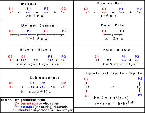
Fig. 176 Survey configurations for DC resistivity surveying.

Plotting raw data

How are apparent resistivities (calculated from measured potentials, currents and geometries) displayed for direct interpretation or for quality assessment? There is one conventional plotting scheme for soundings, while plotting of profiles depends upon the survey configuration.

Soundings

Soundings are used when the earth’s electrical structure needs to be interpreted in terms of layers under a single location at the surface. The electrode spacings are varied symmetrically about a central location.

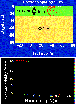
Figure 8. Therefore, data must be plotted as a function of electrode spacing rather than as a function of location. The resulting plot is called a sounding curve, and it arises as shown in this interactive figure (Figure 8). Only current electrodes are shown. Potentials would be measured inside current electrodes using either the Wenner or Schulmberger configurations.

At small electrode spacings current flows only in near-surface regions. Apparent resistivities look similar to the true resistivity of overburden. As current flows deeper, apparent resistivities are influenced by the true resistivities of deeper materials. The sounding curve begins to indicate that there are at least 2 layers under this location. At very large electrode spacings most of the information reflects deeper ground because that is where most of the current is flowing. The completed sounding curve. 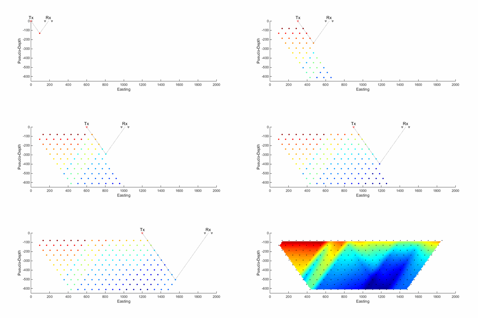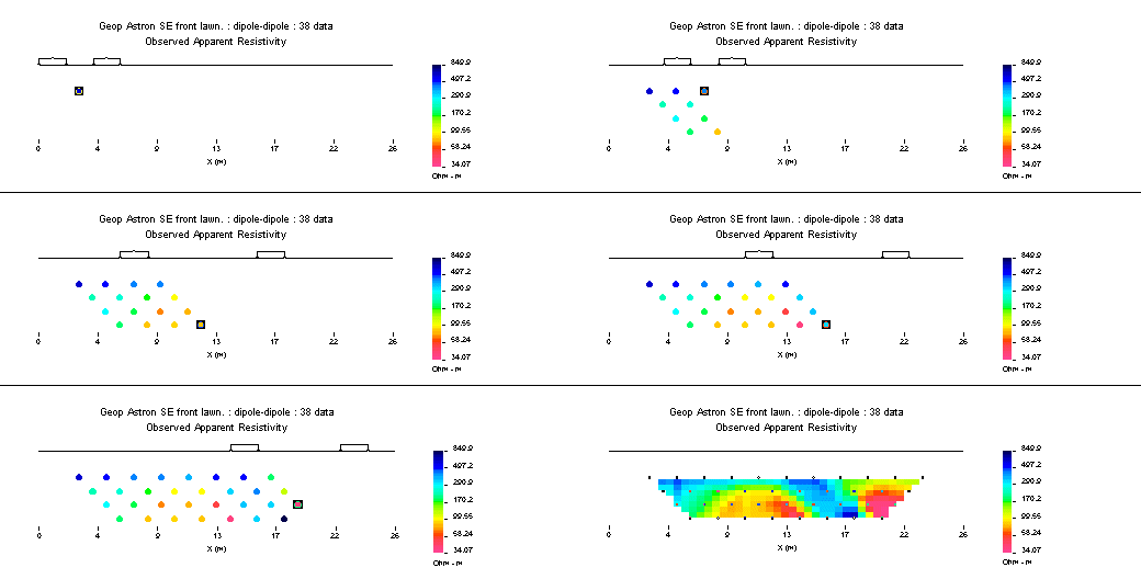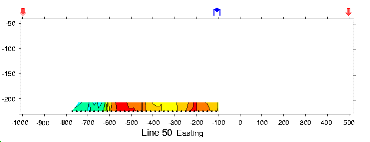Profiling Simple profiling involves moving a fixed array of four electrodes along a survey line. If there are no changes of spacing, then a simple graph of apparent resistivity versus line position would be adequate. A contour plot could be created if there is suitable coverage of the area. Pseudosections: When profiling, potentials are usually measured at several positions for every current source location. Results at wider separations between the potential pair and the transmitter pair provide some information about deeper structures. The conventional method of plotting such results is the pseudosection, so called because it is not a true geological cross- section. Values of apparent resistivity are plotted on the graph as shown in Figures 9 and 10. The vertical axis represents separation distance, NOT depth. When all values are plotted, the result is contoured. Interpretation is tricky and requires some experience. Fig. 177 Figure 9. Plotting a pseudosection of dipole-dipole data: current electrodes are spaced a meters apart (same for potential electrodes), and current-voltage separation is n×a meters (n is an integer). In the animation in Figure 10, the process of gathering and plotting profiling data is illustrated. The survey illustrated involves a dipole-dipole array with \(a = 2\) meters, and \(n = 4\). Figure 10. For each measurement, notice the positions of current electrodes (left pair) and potential electrodes (right pair). Vertical axis of the plotted data is NOT depth; it is the value n, from 1 to 4 in this case. Display the finished contoured pseudosection. Return to the animation. Gradient array: Large scale reconnaissance surveys are sometimes done using the gradient array (Figure 7e above). If the current sources are not moved, then the energizing field is the same for all measurements. There is, therefore, no inherent information about variations with depth, just like the case of gravity and magnetic surveys. Gradient array surveys are often displayed simply by contour plotting the results. Real Sections: There is one variation of the gradient array that provides limited information about structures at depth. It is run under the trade name “real-section,” but the plot is still a “pseudosection” because apparent resistivity data are plotted with no attempt to convert apparent (measured) resistivities into true (intrinsic) resistivities. In the following figures, red electrodes are the current source, and blue electrodes are the potential measurement electrodes. A row of potential measurements at fixed “a” spacing is gathered for each pair of current electrode placements. This is basically a set of seven (in this case) gradient surveys along the same line. At four stages in acquisition, the data look like the following: Figure 11. Although the result is not a "real" section at all, data can be inverted as for any other pseudosection to provide a more legitimate estimate of the true Earth resistivity structure. This example shows data gathered over the San Nicolas deposit in Mexico. After several measurements at one current source spacing. After changing to narrower current spacing and re-doing potential measurements. Over halfway completed. The completed "real-section" pseudosection. Choice of array: Does the choice of array type matter for profiling? Appendix II has a brief comparison of pseudosections and the results of inverting data gathered using the arrays. Processing options Very little processing is applied to most raw resistivity data, other than to convert from apparent resistivities to potentials if that is needed for input to inversion programs. This is accomplished by using the apparent resistivity formula for the array in use, and the known geometric factor. If the current, \(I\), is taken to be 1 (even if it was not 1 Amp in the field), then the result is a normalized potential in units of volts.