Travel times

A seismic wave travelling through an isotropic homogeneous medium will propagate at a constant velocity. Therefore, the time \(t\) required for a seismic wave to travel from source to receiver in a homogeneous earth layer with velocity \(v\) is simply given by the formula

\[t = \frac{d}{v}\]

where \(d\) is the distance travelled in the layer. In a seismic survey we measure source to receiver travel times and use those data to estimate the properties of the subsurface. Basic seismic interpretation methods assume that the earth is composed of a series of uniform layers and attempt to compute the thicknesses, velocities, and sometimes dips of each layer. We will discuss specific techniques for computing layer thicknesses and velocities in the reflection and refraction survey sections. However, we will introduce the concept of travel time computations and how they relate to geometry here, using the example of a two layered earth.

Consider a layer of thickness h and velocity \(v_1\) overlying a uniform halfspace of velocity \(v_2\). A source is detonated at time \(t=0\). We are interested in the waves and arrival times of those waves at a receiver which is located at a distance \(x\) from the source at position \(D\) in the figure below. There are three principal waves that will travel through the earth and arrive at position D. i) direct waves, ii) reflected waves, and iii) critically refracted waves.

The travel time curves for these ray paths are shown below, where the horizontal axis represents distance from the source along the flat surface of the earth, \(x_{crit}\) is called the critical distance, and \(x_{cross}\) the crossover distance. The critical distance is the closest surface point to the source at which the refracted ray can be observed. The crossover distance is the surface point at which the direct and refracted rays arrive at the same time. At offsets from the source greater than the crossover distance the refracted ray will be the first signal to arrive from the source. You can explore these concepts interactively using the Science seismic refraction app. Instructions for using the app can be found here. The following video illustrates the propagation of headwaves and how they relate to the crossover distance

Travel times of visible arrivals are related to the distance between source and receiver (\(x\)), thickness of the layer (\(h\)) and the wave velocities in the upper layer and basement (\(v_1\) and \(v_2\)). Let us denote the arrival times at point \(x\) for the direct, reflected and refracted waves as \(t_{dir}\), \(t_{refl}\) \(t_{refr}\) respectively. These times are given by the following formulas

\[\begin{split}t_{dir} & = \frac{x}{v_1}\\ t_{refl} & = \frac{\sqrt{x^2 + 4h^2}}{v_1}\\ t_{refr} & = \frac{x}{v_2} + \frac{2h\sqrt{v_2^2-v_1^2}}{v_1 v_2}.\end{split}\]

Note that the formulas for the direct and refracted waves are linear in \(x\) but that the reflected arrival time formula is not.

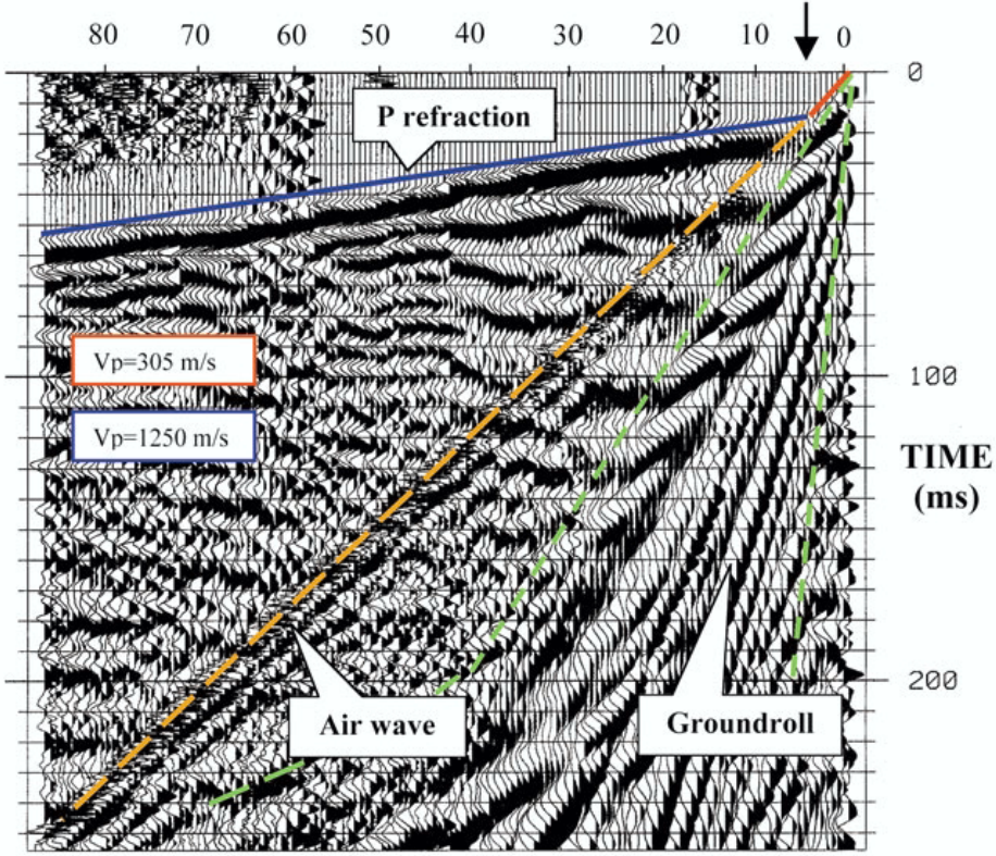
Before moving on, let’s look at an example of how travel times show up in the field. The horizontal axis of the following plot shows offset from a seismic receiver. Each line plots the displacement vs time curve of a geophone at a given offset. The plot clearly shows a set of events moving linearly in time from one geophone to the next.

We will now discuss the computation of traveltimes in more detail. It is important to note here that computing traveltimes for an arbitrary, heterogeneous earth is a complex problem well beyond the scope of this course. However, much insight can be gained by assuming that the subsurface consists of a series of homogeneous layers with horizontal or possibly dipping interfaces.

Refracted ray in a two layered-earth

We need to identify specific ray paths and their associated travel times. Consider an earth composed of a uniform layer with velocity \(v_1\) and thickness \(z\) overlying a medium with velocity \(v_2\). Let \(\theta\) be the critical angle and x denoted the distance between the source at \(A\) and a receiver at \(D\). Let \(x_c\) denote the critical distance.

triangle

From elementary geometry the following relationships hold:

\[x_c = 2z\tan\theta \quad l=\frac{z}{\cos\theta}\]

or

\[\tan\theta = \frac{x_c}{2z} \quad \cos\theta = \frac{z}{l}\]

The travel time is the cumulative time for the wave to traverse the path \(ABCD\). This is \(t=t_{AB}+t_{BC}+t_{CD}\).

Generally time = distance / velocity, so we can write \(t_{AB} = L/v_1 = (z/cos\theta) / v1\), (using \(L\) from just above).

Also, we can note that \(t_{AB} = t_{CD}\) and the distance \(BC\) is \(x-x_c\). So we can now state that \(t=2t_{AB}+t_{BC}\) , or

\[t = \frac{2z}{v_1\cos\theta} + \frac{x-2z\tan\theta}{v_2}\]

velocity triangle

It is convenient to rearrange this slightly differently. Using the definition for critical angle \(\sin\theta=v_1/v_2\), we can make the “velocity triangle”, so expressions for the angle arise directly from simple trigonometry:

\[\cos\theta = \frac{\sqrt{v_2^2-v_1^2}}{v_2}\]

\[\tan\theta = \frac{v_1}{\sqrt{v_2^2-v_1^2}}\]

Use these two relations for \(\cos\) and \(\tan\) in the expression for t above to obtain a useful set of relations.

\[\begin{split}t = & \frac{x}{v_2} + \frac{2z\sqrt{v_2^2-v_1^2}}{v_1v_2} \\ = & \frac{x}{v_2} + t_i\end{split}\]

This simple relation says that the travel time curve is a straight line which has a slope of \(1/v_2\) and an intercept of \(t_i\). This intercept time is the time where the refraction line extends to intercept the \(y\)-axis –above the source position–. This is not a real “time” - it is derived from the graph.

The velocities of the seismic layers and the layer thickness are obtained in the following manner.

1. Plot the times of first arrivals on an time-offset plot (“offset” is distance between source and geophone).

2. The direct arrivals are observed to lie along a straight line joining the origin. The slope of this line is \(1/v_1\), giving the velocity of the upper layer.

3. The refracted arrivals appear as a straight line with smaller slope equal to \(1/v_2\), giving the velocity of the lower layer.

4. For the refracted wave, this intercept time is

\[t_i = \frac{2z\sqrt{v_2^2-v_1^2}}{v_1v_2}\]

so

\[z = \frac{t_iv_1v_2}{2\sqrt{v_2^2-v_1^2}}\]

We therefore can obtain all three useful parameters about the earth, \((v_1, z, v_2)\).

There is another useful point that is observable from the first arrival travel-time plot. We can often discern the crossover distance. Since this is the location where the direct wave and the refracted wave arrive at the same time, we can write

\[\frac{x_{\text{cross}}}{v_1} = \frac{x_{\text{cross}}}{v_2} + t_i\]

Thus

\[x_{\text{cross}}\left(\frac{1}{v_1} - \frac{1}{v_2}\right) = t_i\]

\[\begin{split}x_{\text{cross}} &= \left(\frac{v_1v_2}{v_2-v_1}\right)t_i \\ &= \frac{v_1v_2}{v_2-v_1}\frac{2z}{v_1v_2}\sqrt{v_2^2-v_1^2} \\ &= 2z\sqrt{\frac{v_2+v_1}{v_2-v_1}}\end{split}\]

This can be used as a consistency check, or it can be used to compute one of the variables given values for two others.

Refracted ray in a three layered-earth

The extension to more layers is in principle straight forward. Snell’s law holds for waves at all interfaces, so for a multi-layered medium

\[\frac{\sin\theta_1}{v_1} = \frac{\sin\theta_2}{v_2} = \frac{\sin\theta_3}{v_3} = ...\]

For a three layer case, the algebra is slightly more involved compared to a two layer example because we need to compute the times due to the ray path segments in the two top layers. Consider the diagrams below:

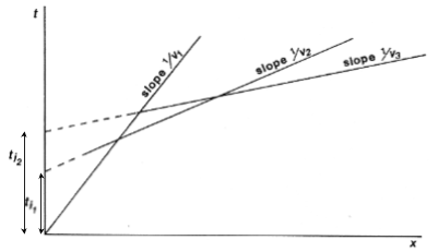
Using arguments that are entirely analagous to the two layer case (above) the travel time for the wave refracted at the top of layer three is given by

\[\begin{split}t &= \frac{x}{v_3} + \frac{2 z_1 \cos\theta_1}{v_1} + \frac{2z_2\cos\theta_2}{v_2} \\ &= \frac{x}{v_3} + t_{i2}\end{split}\]

All quantities are defined in the diagrams, and the angles are

\[\theta_1 = \sin^{-1}\left(\frac{v_1}{v_3}\right) \quad \text{and} \quad \theta_2 = \sin^{-1}\left(\frac{v_2}{v_3}\right)\]

Note that \(\theta_2\) is a critical angle while \(\theta_1\) is not. You can prove the relation for \(\theta_1\) yourself by using Snell’s law at the two interfaces, and recalling that the angle of the ray coming from point \(B\) is the same as the angle arriving at point \(C\). The straight line that corresponds to an individual refractor provides a velocity (from its slope) and a thickness (from the intercept). Thus the information on the above travel-time plot allows us to recover all three velocities and the thickness of both layers.

The travel time curves for multi layers are obtained from obvious extension of the above formulation.

Reflected rays - single layer

Consider the situation to the right, in which there is a source \(S\) and a set of receivers on the surface of the earth. The earth is a single uniform layer overlying a uniform halfspace. A reflection from the interface will occur if there is a change in the acoustic impedance at the boundary.

Let \(x\) denote the “offset” or distance from the source to the receiver. The time taken for the seismic energy to travel from the source to the receiver is given by

\[t = \frac{(x^2 + 4z^2)^\frac{1}{2}}{v}\]

This is the equation of a hyperbola. In seismic reflection (as in radar) we plot time on the negative vertical axis, and so the seismic section (without the source wavelet) would look like.

Two way travel time:

\[t_0 = \frac{2z}{v}\]

Normal Moveout:

\[\Delta t = t(x) - t_0\]

In the above diagram \(t_0\) is the 2-way vertical travel time. It is the minimum time at which a reflection will be recorded. The additional time taken for a signal to reach a receiver at offset \(x\) is called the “Normal Moveout” time, \(\Delta t\). This value is required for every trace in the common depth point data set in order to shift echoes up so they align for stacking. How is it obtained? First let us find a way of determining velocity and \(t_0\).

For this simple earth structure the velocity and layer thickness can readily be obtained from the hyperbola. Squaring both sides yields,

\[t^2 = t_0^2 + \frac{x^2}{v^2}\]

This is the equation of a straight line when \(t^2\) is plotted against \(x^2\). Now, to find \(\Delta T\), we must rearrange this hyperbolic equation relating \(t_0\), \(x\), the \(Tx\)–\(Rx\) offset, \(t\) at \(x\), or \(t(x)\), and the ground’s velocity, \(v\).

\[ \begin{align}\begin{aligned}\begin{split}t^2 &= \frac{x^2 + 4z^2}{v} \\ &= \frac{4z^2}{v^2}\left(\frac{x^2}{4z^2} + 1 \right)\\\end{split}\\\begin{split} t &= \frac{2z}{v} \sqrt{ 1 + (\frac{x}{2z})^2 } \\ &= t_0 \sqrt{ 1 + \left(\frac{x}{vt_0}\right)^2 }\end{split}\end{aligned}\end{align} \]

Apply binomial expansion to get

\[t \approx t_0 \left(1 + \frac{1}{2} \left(\frac{x}{vt_0} \right)^2 \right)\quad if \quad \frac{x}{vt_0} << 1\]

Now, since normal moveout is \(\Delta T = t_x - t_0\)

\[\Delta t \approx \left(t_0 + \frac{t_0x^2}{2v^2t_0^2} \right) - t_0 \approx \frac{x^2}{2v^2t_0}\]

The algebra has only one complicated step–a binomial expansion must be applied to obtain a simple relation without square roots etc.

The approximation is valid so long as the source-receiver separation (or offset) is “small” which means much less than the vertical depth to the reflecting layer (i.e. \(x << vt_0\)). The result is a simple expression for normal moveout.

Each echo can be shifted up to align with the \(t_0\) position, so long as the trace position, \(x\), the vertical incident travel time, \(t_0\), and the velocity are known. Velocity can be estimated using the slope of the \(t^2\)–\(x^2\) plot, or with several other methods, which we will discuss in pages following.

Travel Time Curves for Multiple Layers

If there are additional layers then the seismic energy at each interface is refracted according to Snell’s Law. The energy no longer travels in a straight line and hence the travel times are affected. It is observed that for small offsets, the travel time curve is still approximately hyperbolic, but the velocity, which controls the shape of the curve, is an “average” velocity determined from the velocities of all the layers above the reflector. The velocity is called the RMS (Root Mean Square) velocity, \(v_{rms}\).

The complex travel path of a reflected ray through a multilayered ground. (b) The time–distance curve for reflected rays following the above type of path. Note that the divergence from the hyperbolic travel-time curve for a homogeneous overburden of velocity Vrms increases with offset.

As outlined in the figure above, the reflection curve for small offsets is still like a hyperbola, but the associated velocity is \(v_{rms}\), not a true interval velocity.

For each hyperbola:

\[t \approx \frac{\left(x^2 + 4z_n^2 \right)^2 } {v_n^{rms}}\]

By fitting hyperbolas to each reflection event one can obtain \(t_n,v_n^{rms}\) for n = 1, 2, … The interval velocity and layer thickness of each layer can be found using the formulae below:

\[ \begin{align}\begin{aligned}v_n \approx \left[ \frac{(v_n^{rms})^2 t_n - (v_{n-1}^{rms})^2 t_{n-1} }{t_n-t_{n-1}} \right]\\\Delta z = z_n - z_{n-1} = v_n \left( \frac{t_n - t_{n-1}}{2} \right)\end{aligned}\end{align} \]

These formulae for the interval velocity and thickness of the \(n^{th}\) layer are directly obtainable from the definition of \(v_n^{rms}\) given above. The RMS velocity for the \(n^{th}\) layer is given by:

\[v_n^{rms} = \sqrt{\frac{\sum_{i=1}^{n} v_i^2 \tau_i}{\sum_{i=1}^{n} \tau_i}}\]

where \(v_i\) is the velocity of the \(i^{th}\) layer, and \(\tau_i\) is the one-way travel time through the \(i^{th}\) layer.