Interpretation

In this section, we use a real-world example to illustrate the use of electromagnetic (EM) methods. In this industrial reclamation case study, the interpretation of EM data had proven useful in characterizing the sub-surface and answering the following questions:

1- What is the thickness of the mixed fill layer (i.e. what is the depth to till)?

2- What is the distribution of buried objects? Many objects are thought to exist, possibly ranging in size from small pieces of industrial trash, to railway lines, reinforced concrete building foundations, and buried tanks.

3- Can geophysics contribute any information about the extent of hydrocarbons within the top layer, which consists of a wide range of fill materials?

4- Where is fill material dominated by wood waste, making ground unfit to support structures?

Background

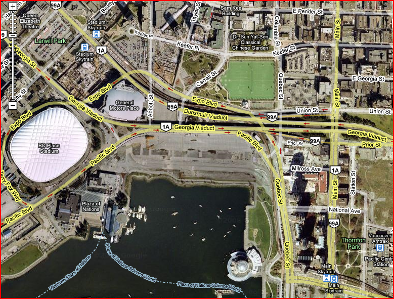
Fig. 148 Recent satellite image over the old Expo site, Vancouver, BC.

The field site in question is an urban area with a complex industrial history located on the outskirt of downtown Vancouver, Canada. The same site had been used for the 1986 World Exposition on Transportation and Communication, also known as the Expo site. Following the Expo, the city undertook excation work prior to the construction of public space [REF NEEDED]. The actual field site was fully remediated by the end of 1991, as summarized by the closure report prepared by Golder Associates Ltd.

Historical Land Use

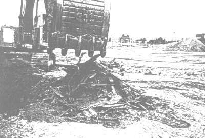
Fig. 149 Excavated wood debris below the Expo site.

The land had been used by several insdustries over the years, laying down pipes, railroads, cables and several utility buildings. The history of industrial activity is fairly complex, and covers over 100 years. For example, Fig. 149 shows some of the wood waste mixed in with the fill under the pavement at this location. More details about the history are available through the few engineering documents presented below:

1902. Before 1902, there were wood processing and storage facilities in the area. During that period, the original shoreline was moved from the north edge of our site to the south edge using a wide variety of fill materials including wood chips, logs, and construction debris. 1936. After 1902 there was a gas manufacturing plant with storage facilities, an oil house, an auto repair garage, and a substation maintenance facility. The gas plant left some quantities of ammonia, phenolics, cyanide, oxides, and light hydrocarbons, as well as other miscellaneous waste. The substation maintenance shop included a sump in the floor into which dielectric fluids from capacitors and transformers was drained. Oil from this sump was piped to the oil house for treatment and recycling. This oil house included large tanks, at least one of which was underground. There was also the Viaduct traffic overpass crossing over the central portion of our site, and associated support foundations may well have been left in the ground when the viaduct was later removed. 1952. Between 1910 and 1960 there were several different railway lines laid at various orientations across our field site. 1961. Sometime in 1969 or 1970 as much as several thousand gallons of oil was spilled on to the shop floor because a valve had been accidentally left open over a weekend. 1974. After 1974, a fuel depot, bus wash and several underground storage tanks existed. These were demolished for the most recent use, which was a parking lot for a near by Exposition.

Stratigraphy

Based on monitoring wells, boreholes and trenching the north-south cross section shown to the right was constructed. The five primary stratigraphic units in the area of interest can be described as follows.

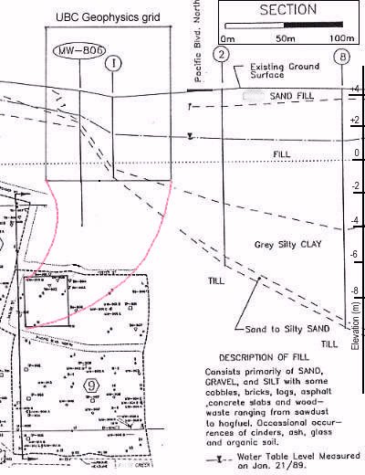
Fig. 150 Known stratigraphy from monitoring wells, boreholes and trenching.

• The top half metre consisted of two layers of very hard pavement.

• The fill below was very variable, consisting mainly of mineral fill, but with considerable quantities of other materials, including buried metal and concrete, wood waste, construction debris and gravel fill. Individually, these materials have a wide range of physical and geotechnical properties, and when used as fill, bulk (averaged) properties would also range widely. Identifying elevation highs and lows may provide some insight as to where more (or less) compressible fill materials existed.

• The next unit below the artificial fill was a sandy silt (or silty clay in some areas), ranging between zero and one metre thick. The deepest layer penetrated by boreholes was a very dense gray sandy silt, with some gravel and traces of clay - basically a till.

• The depth to this till is moderately well-constrained under the profile to the west of the field site.

• Sedimentary bedrock was reportedly deeper than 20 m.

Hydrogeology

The depth to the water table was known to vary between 1 and 3 m, with flow generally towards the South West. The principle hydrostratigraphic unit (fill) was generally highly permeable but with isolated regions that appeared to block flow through this aquifer. Transformer oil contaminated with polychlorinated biphenyl (PCB) was found in boreholes and test trenches floating on the water table 2 m to 3 m below ground surface in some parts of the northern half of the field site.

Buried Metal and Objects

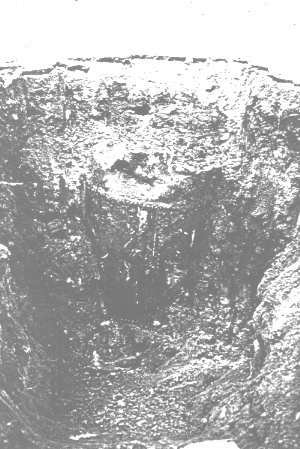
Fig. 151 Buried oil tankIn two of the test pits, high inflows of water (and some oil) were observed in zones of coarse wood waste characterized by open voids up to 10 cm in size

Many kinds of buried objects were encountered in the fill layer. There was much buried metal including wires, tanks, and other known and unknown objects. Fig. 151 shows a buried tank found at test pit 28. A buried oil sump was also expected in the location of the oil house associated with the maintenance shop near the North edge of the site. It is also possible that re-bar reinforced concrete foundations of buildings or supports for the old traffic Viaduct could be encountered. There were also old railways, although no evidence of the iron rails themselves was found in trenches or boreholes. Above ground, there are several lamps, and a chain link fences surrounds our study area on three sides. The lamps are expected to be connected to underground wiring since they are not fed by overhead wires.

Hydrocarbons

Early in our work, a monitoring well was discovered to have up to 20 cm of oil floating on the water table, containing concentrations of PCB’s higher than the local special waste regulations permitted. As a result, an investigation program was conducted to delineate the areal extent and thickness of the oil, to assess the PCB concentrations, and to locate any potential remaining sources of oil such as underground tanks. The investigation involved excavation of 36 test pits, and collection of 7 oil samples, 58 soil samples, and 10 water samples. Details about all boreholes and test pits are contained in a separate report. We recommend that geophysical surveys be conducted in order to further delineate contaminated zones, and to locate subsurface features that might be associated with oils. This is because the largest concentrations of PCB’s were found in black stained soil inside or adjacent to buried pipes and transformer parts. This increases the importance of investigating all geophysical anomalies that could be buried metal debris.

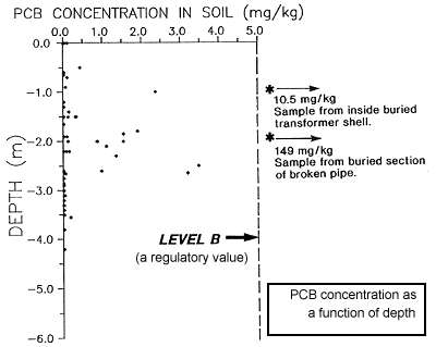
Fig. 152 PCB samples measured at the Expo site.

PCB concentrations were measured in 58 soil samples with results as shown in Fig. 152. Most of the contamination was found within the depth range of 1m to 3m, which corresponds to the fluctuation of the water table. Samples from five standpipe locations were used to characterize the oil itself, in terms of carbon distribution, viscosity, specific gravity and flashpoint. The oil / water contact was found to be blurred even after samples gathered from standpipes had been left to stand for 24 hrs. The diffuse layer between oil and water was inferred to consist of emulsified oil possibly resulting from weathering due to microbial activity over the extended time period. Note that this probably has important implications for detection using geophysics for at least two reasons: i) the interface between water and oil is not manifested as a distinct transition in physical properties, and ii) there are in effect three fluids rather than two - water, oil, and the mixture.

Survey

The Geonics EM-31 instrument is used to map variations of electrical conductivity within the top 3 to 6 metres of the sub-surface. This chapter of our report summarizes survey design and results obtained. Detailed interpretation was not one of our contractual oblications. Survey design

For EM-31 surveys, rapid acquisition of spatially dense data sets is usually the most important requirement. When searching for discrete targets, the most important design consideration is to avoid spatial aliassing. For small 3D targets a tightly spaced grid would be required. For 2D targets (such as buried utility pipes), data spacing along profile lines would likely be tighter than spacing between lines, assuming lines can be placed perpendicular to target orientation.

At our field site, EM-31 data were gathered on a 2m grid resulting in measurements of in-phase and quadrature response at 2600 stations. Since the instrument response to elongated buried objects depends upon the orientation of the instrument, two complete data sets were gathered, with the instrument’s 3.66 m boom oriented both in north-sourth and east-west directions.

Both complete data sets are presented in Table 11. They were recorded using the “normal” vertical dipole coil orientation with the instrument held 1 m above the ground.

Table 11 EM 31 data the Expo site

Fig. 153 : \(\sigma_{app}\) map from the EW orientation

Fig. 154 : \(\sigma_{app}\) map from the NS orientation

Fig. 155 : In-phase map from the EW orientation

Fig. 156 : In-phase map from the NS orientation

Apparent conductivity data are presented in units of milliSeimens per m (mS/m) using a rainbow colour scale with banding so that values and local trends are both visible. Corresponding in-phase data are in percent of primary field strength, and are presented using a bimodal colour scale since results are generally interpreted qualitatively to identify buried metal rather than quantitatively in terms of ground material properties.

Processing

Since data were gathered using two different instrument orientations, it is easy to supply averaged and differenced data sets. Averaged and differential maps are presented in Table 12. The effect of averaging data from two orientations is to smooth responses, emphasizing regions where ground is more uniform. The objective of differencing data from two orientations is to emphasize features that depend upon instrument orientation. For apparent conductivity data the result is that linear and small 3D targets are more clearly decerned. Click the following small images to display larger versions of each image.

Table 12 Processed data at the Expo Site

Fig. 157 : Averaged EW and NS \(\sigma_{app}\) map

Fig. 158 : Differenced EW and NS \(\sigma_{app}\) map

Fig. 159 : Averaged EW and NS In-phase map

Fig. 160 : Differenced EW and NS In-phase map