Frequency Domain Data

Nature of the total field

Consider a frequency domain source. This could be a loop on the ground or in the air.

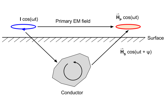
1. The primary field is harmonic \(\cos(\omega t)\). At the receiver, the primary field can be written as \(\vec{H}_p \cos(\omega t)\).

2. The currents induced in the conductor will also be harmonic with the same frequency \(\omega\). They will, however, have a different phase. The resultant secondary field from these currents must also have the same frequency dependence. Hence, the secondary field can be written as \(\vec{H}_s \cos(\omega t + \psi)\), where \(\psi\) is a phase angle.

At the receiver, we observe the sum of the primary and secondary fields, which is given by

\[\vec{H}_{total} = \vec{H}_p \cos (\omega t) + \vec{H}_s \cos (\omega t + \psi)\]

The Phase of the Secondary Field

If the primary field is harmonic with frequency \(\omega\) then the secondary field is also harmonic. The secondary field will have a different phase than the primary; it will lag the primary field by angles between 90° and 180°. The amount of phase difference is diagnostic of the conductivity of the body.

1. The primary current varies as \(\cos(\omega t)\) and hence the primary magnetic field also has this same dependence. (The primary field is in-phase with the current).

2. At the conductive body the EMF (induced voltage) is

\[\mathcal{E} = - \frac{d \phi_B}{dt}\]

If the primary current varies as \(\cos(\omega t)\) then the flux, \(\phi_B\) also varies as \(\cos(\omega t)\), while \(\mathcal{E}\) varies with \(\sin(\omega t)\). That is, the EMF lags the primary by \(\pi/2\).

3. The body in which the induction is occurring can be represented as a circuit element with self-inductance \(L\) and a resistance \(R\). Through the laws of electromagnetic induction, the time varying currents that are set up in the conductor suffer a further lag

\[\phi = \tan^{-1} \left( \frac{\omega L}{R} \right)\]

4. As a result the secondary field lags the primary by a total amount

\[\psi = \frac{\pi}{2} + \tan^{-1} \left( \frac{\omega L}{R} \right)\]

Note:

1. For a resistive body (or for very low frequency) \(\phi \rightarrow 0\) so the secondary field is only \(\pi/2\) out of phase with the primary field. The response from a weak conductor will be in the out-of-phase component of the measured signal.

2. For very conductive bodies (or for very high frequency) the secondary field becomes nearly \(\pi\) (180°) out of phase with the primary. Since \(\cos(\omega t + \pi ) = -\cos(\omega t)\), the response due to a good conductor will be in phase with the primary but reversed in sign.

Measurement of Secondary Fields

The easiest quantity to measure is some component of the total field. However, from an interpretation viewpoint, we are interested in the secondary field produced by the body. Unfortunately the primary field is generally very much larger than the secondary field and hence if we measure their sum then we are faced with finding, and interpreting, a small signal in the presence of a large signal. It would be more advantageous to measure the secondary field directly. This can be done in two ways:

1. One can have a “bucking” coil or “compensator” that provides a magnetic field at the receiver, which has the same amplitude and phase as the primary field but is in the opposite direction. As a result \(\vec{H}_p\) is annihilated at the receiver, (eg. aircraft systems. Lab systems, EM-31).

2. There can be a direct link between the transmitter and receiver through a connecting cable. This allows for a phase reference and hence the field, which is adjusted for amplitude loss due to geometrical spreading, can be subtracted from the measured signal.

In-Phase and Quadrature Phase

With the removal of the primary field the reading at the receiver pertains to the secondary field. What is generally presented as data is the ratio of the secondary field to primary field for a particular component of the field. (Remember that data could be magnetic fields measured with a magnetometer or voltages measured with a coil.) The data will be ratio of the secondary field to the primary field. Let the primary field be \(H_p \cos(\omega t\)). The secondary field is \(H_s \cos(\omega t + \psi)\) and can be written as

\[\begin{split}H_s \cos(\omega t + \psi) = H_s [ \cos(\omega t) \cos(\psi) - \sin(\omega t) \sin(\psi) ] \\ = [H_s \cos(\psi)] \cos(\omega t) - [H_s \sin(\psi)] \sin(\omega t)\end{split}\]

The first term has the same phase as the primary field and is referred to as the “in-phase” response. This is also sometimes referred to as the “real” part of the response. Such terminology is used due to derivations are made in terms of complex quantities.

In-phase:

\[\frac{H_s \cos(\psi)}{H_p}\]

The second term is the “out-of-phase” part or quadrature phase.

Out-of-phase:

\[\frac{H_s \sin(\psi)}{H_p}\]

This term is also referred to as the “imaginary” part of the response. Unfortunately, different words refer to the same thing. Don’t be confused. Similar terminology is summarized as follows:

In-Phase	Out-of-Phase
Real	Imaginary
	Quadrature

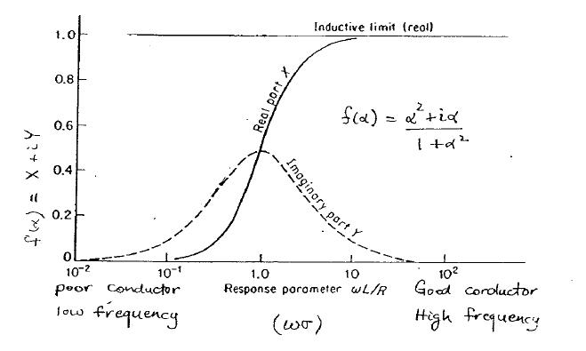
Since both in-phase and out-of-phase quantities are small, their values are usually given in ppm (parts per million). Insight regarding the expected value of the In-phase and Out-of-phase components can be obtained by examining the response of a single loop of wire (of resistance \(R\) and inductance \(L\). The ratio \(H_{secondary} / H_{primary}\) or ( \(V_s/V_p\) if the receiver is a coil) is given by

\[\frac{H_S}{H_P} = \text{(Coupling Coefficients)} \cdot f(\alpha)\]

where \(\alpha = \omega L / R\). A plot of \(f(\alpha)\) provides considerable insight into electromagnetic data. Such a plot is probably one of the most important plots in electromagnetic induction. \(f(\alpha)\) is a complex number and has real and imaginary parts.

Remark: for those familiar with complex numbers, the coupling coefficients are given by:

\[f(\alpha) = \frac{\alpha^2 + i \alpha}{1 + \alpha^2}\]

The coupling coefficients depend upon the orientation of the transmitter and receiver as well as the geometry of the target body.