Survey¶

Having decided that magnetic susceptiblity is a diagnostic property for our problem, the next step is to choose an appropriate survey. Designing an effective magnetic survey requires choosing the field instrumentation, as well specifying an adequate survey layout. Surveys over simple and complex scenarios are provided to highlight some of the possible complications encountered in real-life applications.

Further details about instrumentation are provided later in this section. For now it is only necessary to understand that magnetic instruments can measure: (a) the total magnetic field \(|\mathbf{B}|\). (b) an individual component of \(\mathbf{B}\), such as \(B_x\), \(B_y\) or \(B_z\) (c) a gradient of the magnetic field

Of the above choices, by far the most common is the measurement of the total magnetic field. However, the same principles of survey design discussed below apply to all of these measurements, in particular the total field anomaly datum which is the projection of the anomalous field onto the direction of Earth’s field.

Survey Design¶

A key component of any geophysical experiment is the design of an effective survey that can optimize the amount of information gathered with the least amount time spent in the field. Here are few important parameters to keep in mind:

Coverage: the survey area must be large enough to capture the anomalous signal

Sample interval: the data must be sampled finely enough so that the anomalous signal is captured with good fidelity.

These concepts are clarified below:

Coverage¶

The area over which the magnetic data are collected must be of great enough extent to capture the anomalous signal. If only part of the signal is measured it will be difficult to image the causative body or structure. Fig. 37 compares two surveys over a dipping plane [ Strike: \(315^{\circ}\) , Dip: \(45^{\circ}\) ]. Both surveys used the same number of stations, hence the data acquistion cost would have been about the same. The example is small scale, with a plane being only 3 x 3 meters but the survey design principles do not change with scale of the object.

In the first case (a), the survey area is only 2m x 2m and it barely reaches the edge of the buried plane. Little can be said about its horizontal extent. The survey managed to measure the peak magnetic anomaly, but nothing can be inferred about a possible geometry of the plane.

In the second case (b), the survey area is 8m x 8m and the anomalous field has decayed to zero at the edges of the survey. This is ideal. The survey area extends far away from the peak values and approximately delineates the edges of the magnetized object. A trained eye could potentially recognize the signature of a dipping magnetic plane. (Of course we will do better by inverting the data!)

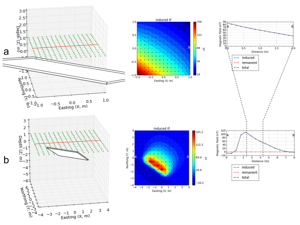
../../_images/magnetic_coverage.png — Fig. 37 : (a) \(4\;m^2\) and (b) \(64\;m^2\) magnetic surveys over a dipping magnetic plane. The wider survey successfully captured the full amplitude of the magnetic anomaly.¶

Sampling interval¶

The sampling interval, or distance between observation points, is also important for a meaningful interpretation of magnetic data. Two surveys with variable station spacing over a magnetic rod are presented in Fig. 38. The data acquired at a lower resolution gives little indication about the orientation of the magnetic rod. Only when the sampling interval is decreased can we distinguish a linear feature striking at \(30^{\circ}\) N.

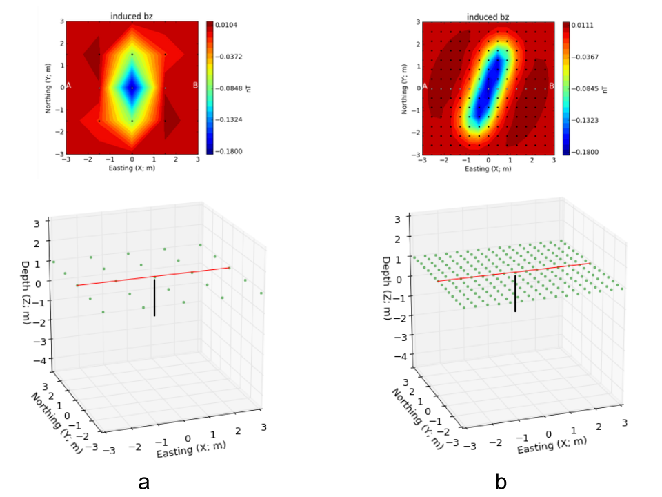
../../_images/magnetic_sampling.png — Fig. 38 : Magnetic surveys at (a) \(0.4\;m\) and (b) \(1.2\;m\) station spacing acquired over a magnetic magnetic rod oriented \(30^{\circ}\) N.¶

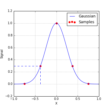
../../_images/Sampling_Frequency.png — Fig. 39 : Rule of thumb for sampling frequencies¶

The above example illustrates a “General Rule of Thumb for Sampling Interval”: In order capture the details about the anomalous field, data should be acquired so that there are at least about 3 points per halfwidth of the signal. This is illustrated in Fig. 39. A more specific analysis, from a time series viewpoint, is that any frequency component of the signal needs to be sampled at least two times in each period. For our purposes, sampling the fields finely enough so that you produce the main features of the anomalous field is sufficient.

Important point: Note that survey area that is needed to capture the anomaly, and the sampling interval both depend upon the depth of burial of the object. If the object is small and buried very close to the surface then the footprint of the object is small. The station space is correspondingly reduced.

Student Exercise: Experiment with burying a prism. Using the magnetic_app, place the object at different depths and assess what your estimates of survey area and sampling interval should be. In preparation for a future exercise, look at the relationship between the halfwidth of the anomaly and the depth of burial.

Base Station¶

An important component of the survey is setting up a base station. A base station is generally set up in the vicinity of the survey area, and away from known magnetic sources like powerlines. The magnetometer at the base station records continuously during the survey period and serves as a reference for later processing of the magnetic data where we attempt to remove the daily variations of the inducing field due to external sources.

Line profiles for a range of situations¶

Magnetic surveys are (almost) always carried out over an area of interest. In some instances however the geology is 2D and hence a single line profile that is perpendicular to the strike of the geology contains the essential information about the buried bodies. The following examples are instructive in that they show how different such line profiles can be over different parts of the earth.

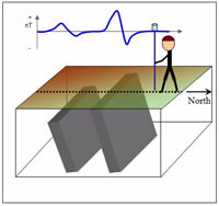
Recall that the anomaly pattern recorded over any given target depends upon latitude, target orientation, profile orientation, remanent magnetization of the target, and possible superposition of adjacent targets. To illustrate, here we show the anomaly recorded over two dykes buried at different depths. The dykes are assumed to extend to very great distances into and out of the page (they are 2D targets), and north is to the right (you are looking west), except in figure 3. The sketch to the right illustrates the situation. The figures below show how data over these dykes will depend on latitude, line orientation, target orientation, and so on. On the graph of the line profile data, note the changes in vertical scale as well as the changes in shape of the graph.

1.	At mid-northern latitudes (45°) the assymetric anomaly has the low end pointing north. Buried dykes are oriented east-west.
2.	At mid-southern latitudes (45°) the anomalous "low" is on the south side.
3.	If buried dykes point north-south so that the survey line runs east-west, the anomaly recorded is very different.
4.	At the magnetic poles, anomalies are symmetric. (Note values for inclination and strike.)
5.	At the magnetic equator, anomalies are also symmetric, but opposite those at the magnetic poles.
6.	If you survey along a line that is at 45° to (rather than perpendicular) the buried 2D target, the anomaly is again very different.
7.	If the shallower body included some remanent magnetization, the anomaly would now consist of the sum of induced and remanent magnetic fields. Compare to example 2., the "normal" anomaly in the southern hemisphere.

	Model earth has two 2D dykes both with susceptiblity k = 15 x 10³.

Working with complex structures¶

In previous sections we learned what the anomalous magnetic field will be over a buried dipole and over extended bodies of uniform susceptibility, and how those ideas apply to geologic structures that have a uniform susceptibility. In general however, the earth is complex and the rocks have variable susceptibility. We simulate the anomalous magnetic fields in the following manner:

Describe the subsurface as a collection of prismatic cells, each of which has its own uniform susceptibility.
The response of a single rectangular cell with constant susceptibility in an arbitrary magnetizing field can be calculated using expressions from the literature. (Think about each cell as being a magnetic dipole.)
The principle of superposition holds. At each location where a measurement is made, the responses from the individual cells are be added up to yield the total response.

The concept is illustrated in the following eight figures selected with the buttons.

1.	First "discretize" the subsurface under the area in which we are interested.
2.	One cell of susceptible material in the cellular subsurface	4.	Five susceptible cells in the descretized earth
3.	Resulting magnetic anomaly at 50^o magnetic north.	5.	Resulting magnetic anomaly at 50^o magnetic north.
		6.	The same data set. Not knowing what caused the anomaly, could you tell where susceptibile blocks are, and how susceptible they are?
7.	A complicated earth with all cells susceptible to some degree.	8.	Resulting data over the complicated earth at 50° magnetic north.

Here again are the data generated from the single block, the 5 blocks and the continuous Earth models:

1. Total field magnetic anomaly over a single block with susceptibility of 0.1 SI units (corresponds to point 2 in the previous figure).

2. Total field magnetic anomaly over five blocks with varying susceptibility (corresponds to point 6 in the previous figure).

3. Total field magnetic anomaly over a volume with all cells having some finite susceptibility (corresponds to point 8 in the previous figure).

The following table gives access to model, mesh and data files associated with these 3 models (uniform earth, 1 block, 5 blocks) for use with UBC-GIF modeling and inversion code MAG3D. The MeshTools3D program is used to view 3D models. The filename extensions will be understandable to those familiar with use of these codes. See MAG3D in IAG’s Chapter 10, “Sftwr & manuals” .

Model	model file	location file	mesh file	data file
Single block:	block_sus	block_sus_loc	block_msh	block_mag
Five block:	block_5_sus	block_5_sus_loc	block_msh	block_5_mag
Continuous earth:	v_sus		v_msh	v_mag

Instrumentation¶

A measurement of the magnetic field at any location will involve either recording the amplitude of the field or one of its three components. Instruments are deployed on the ground, in the air (helicopters and fixed wing aircraft) and in space-borne geophysical platforms. Instrument types commonly used are outlined very briefly as follows:

Total Field magnetometers These instruments measure the amplitude of the magnetic field. The two most common devices are the proton precession and the cesium vapor magnetometers.

Proton Precession Magnetometer¶

This instrument was the most common type before the mid 1990’s. It measures the amplitude of the magnetic field which is sometimes referred to as the Total Field Intensity (TMI).
Advantages: Sensitive to 1 nT, small, rugged & reliable, not sensitive to orientation.
Disadvantages: Takes >1 sec to read, sensitive to high gradients.
The measurement process is related to nuclear magnetic resonance (NMR). A proton source (possibly as simple as a volume of water) is subjected to an artificial magnetic field, causing the protons to align with the new field. When the artificial field is removed, the protons precess back to their original orientation and their precession frequency (called the Larmor precession frequency) is measured. That frequency, \(f\), is related directly to the strength of the earth’s field, (\(B_e\)), according to the equation below. The parameter, \(\gamma_p\), is the ratio of the magnetic moment to spin angular momentum. It is called the gyromagnetic ratio of a proton and is known to 0.001%; \(\gamma_p = 2.67520 \times 10^8 T^{-1} s^{-1}\).

\[f= \frac{\gamma_p B_e}{2 \pi}\]

Cesium (or optically pumped) magnetometer:¶

The physics behind this type of sensor is related to that of the proton precession sensor, but it is more complicated. Although it is more expensive than the above two sensor types, it is now the most commonly used system for small scale work because it is 10 to 100 times more sensitive than the proton precession magnetometer.
The measurement process makes use of the gyromagnetic ratio of electrons and of the quantum behavior of outer-shell electrons of some elements (e.g. cesium). In this case, the relevant gyromagnetic ratio is known to 1 part in 10⁷, and frequencies are near 233 khz, so these instruments are sensitive to 0.01 nT.
Advantages: More rapid readings, 1 or 2 orders of magnitude more sensitive, works in high gradients.
Disadvantages: Optical pumping won’t work when parallel or perpendicular to the magnetic field direction (solved with multiple sensors), ans also more expensive than proton precession.

3-component magnetometers¶

Some sensors can record the magnetic field in a particular direction and hence combining three of them in an orthogonal framework allows three components of the magnetic field to be recorded. A principle challenge in using these in field surveys is that the instruments need to be consistently aligned at the various stations. This means knowing the orientation of the instrument to within a small fraction of a degree. There are two main types of component magnetometers: fluxgates and squids. The fluxgates can be made small enough to be put into a borehole.

Fluxgate Magnetometer¶

The fluxgate magnetometer was developed during WWII to detect submarines. It measures the magnetic field in a specific direction determined by the sensor’s orientation. A complete measurement of the field requires three individual (Cartesian) components of the field ( such as \(B_x\), \(B_y\), \(B_z\) ).
It is generally difficult to get leveling and alignment accurate. Sensor accuracy is 1 nT so orientation must be known to within .001 degrees.

SQUIDS¶

(Superconducting Quantum Interference Devices): These are very sensitive, and are currently more common in laboratories that work on rock magnetism or paleomagnetic studies. However, they are beginning to be used in the field, and more applications will become evident in the coming decade (2000 - 2010).

Magnetic Gradiometer¶

These instruments use two sensors (any of those mentioned above) to measure vertical or horizontal gradients.
They often employ two cesium magnetometers separated by about 1 m.