The problem of estimating a reasonable earth model (i.e. a quantitative
distribution of one or more physical properties based upon recorded data) is
known as the geophysical inverse problem. Various methodologies for performing
geophysical inversion have been developed. There are two broad classes of
inversion: “Parametric” methods and “Generalized” inversion methods.
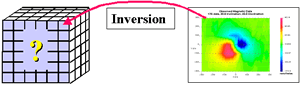
Fig. 5 Inversion: estimating a model based upon measured data and some understanding of the setting
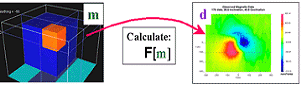
Fig. 6 Forward modelling: calculating data based upon a known earth model
These inversion methods involve finding a model of the earth which is
described using only a few parameters. The solutions require that there be
fewer parameters than there are data values so that the problem is formally
“over-determined.” A few examples of parametric models are:
Buried object: parameters could be depth to a sphere (or cylinder), a radius of a sphere or radius and length of a cylinder, and the physical property contrast between the object and host rocks.
Layered earth: parameters are layer thicknesses and physical property values.
A buried sheet: parameters might be depth to the top of sheet, it’s dip, strike, thickness, and the physical property contrast between the sheet and host rocks.
This second class of inversion methods allows the earth’s model to be more
realistically complex, which means that more parameters than data points are
permitted. These problems are non-unique and require that other information be
incorporated. A work-flow procedure is required and here we highlight a few of
the main components:
Represent the earth with many cells so that complex distributions of
physical properties can be simulated. In practice, the earth is divided into
thousands or millions of cells of fixed geometry. Each cell has a constant,
but unknown, value. The parameters we seek are the physical property values
for these cells. Be able to simulate the field observations if they were
acquired over this model.
Estimate uncertainties in the observed data and design a metric that can be
used to decide when data have been adequately fit.
Design a model objective function. This is a mathematical quantity which
measures the “size” of any solution. It is a single number. A priori
information about the earth can be incorporated into the objective function.
Usually the model objective has different components.One will make it “close”
to a supplied reference model, others may control “smoothness” in various
spatial directions. Models that minimize the objective function are good
candidates for interpretation since they will generally have minimum structure
and tend to reveal the important large scale structure and be good choices .
Use numerical optimization to find a solution that adequately fits the data
and minimizes the model objective function. This yields a solution that is a
good candidate for interpretation.
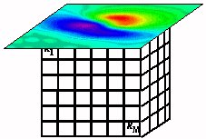
Fig. 7 The earth model is a fixed distribution of cells, each with an adjustable value of the physical property. Measured data are shown on top.
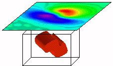
Fig. 8 An inverted model that has minimum structure and acceptably reproduces the data. The generated data from the model are shown on the upper surface and it can be compared with the observed data in the previous figure.
In practice a number of inversions, perhaps with different objective
functions, and different assignments of uncertainties on the data, should be
carried out so the interpreter has some insight about the range of earth
models that can acceptably reproduce the field data. Error statistics about
the data will determine how closely the reproduced data matches the real
measured data.
More detail about inversion and the workflow process is provided in inverse
theory section of the GPG.