Processing

This section focusses on the the temporal and spatial correction of magnetic data prior to the interpretation phase. In most cases, these processing steps are completed by the acquisition team, providing both the raw and processed data as a final product.

Removal of time variations

Earth’s magnetic field changes over time for a variety of reasons. If the changes in earth’s field have an amplitude that is significant compared to our anomalous signal, then we need to correct for the observed temporal variations. The general procedure is to establish a base-station which is fixed in location and continually measures the magnetic field. Each datum acquired by the roving sensor is also time-stamped. The assumption is then made that the changes in the Earth’s magnetic field caused by these natural sources have a long enough spatial wavelength that they are same at any point on the survey grid. Field data, corrected for these time variations, is obtained through the following subtraction process

\[\Delta \textbf{B}(t) = \textbf{B}_{obs}(t) - \textbf{B}_{base}(t)\]

The Geological Survey of Canada geomag page can provide graphs of diurnal variations observed at any of 11 magnetic observatories in Canada, for any day in the most recent 3 years.

Fig. 41 : Adapted from NRC

Removal of regional trends

In order to interpret magnetic data in terms of features and structures at depth, the anomalous field caused by buried features of interest must be isolated. In other words, we must try to remove the contribution to the measurements made by the earth’s field and also from geologic features larger than the actual survey area. That is, we want to remove a regional field. If we designate magnetic fields as B, then we want to perform the following

\[\textbf{B}_{a} = \Delta \textbf{B} - \textbf{B}_{regional}\]

Estimates of the regional field may be obtained using:

• the IGRF

• a constant value selected by the interpreter (when survey areas are small);

• a more sophisticated polynomial (map) generated by a computer using least squares (or other) analysis of data;

• it is also possible to use inversion at a large scale to define a regional field.

To illustrate the process, when data are collected along a line, the removal of a regional trend can be managed graphically, as shown here:

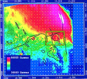
Clearly this process involves some degree of subjectivity and will depend upon how you draw a line that separates the desired “signal” from the background. The situation becomes more complicated for magnetic maps (data collected over an area) where the causative bodies have complicated shapes and variable dimensions. Nevertheless, removing an approximate regional field can be of critical importance in isolating an anomaly for further processing as maps or input into an inversion. The following is an example showing the regional magnetic map and a local anomalous field taken from a survey in central British Columbia. The area is Mt. Milligan, which has recently opened up as a mine. In the large-scale map the dominant feature is the magnetic signature of the mountain. Of interest is a (2km x 2km) segment of that map. A large-scale regional field is estimated, subtracted from the observed data, and the results are shown in a second window. The magnetic feature observed in that map is related to the ore body.

Regional field. Airborne magnetic data gathered a 25 square km area around a mineral deposit in central British Columbia. Some geological structural information is shown as black lines. The monzonite stock in the centre of the boxed region is a magnetic body, but this is not very clear in the data before removing the regional trend. Local anomalous field. Anomalous total magnetic field strength in the boxed area of the large-scale map, after the regional SW-to-NE trend has been removed. Now the signature of the monzonite stock is more clearly visible.

Reduction to Pole

Reduction to pole is a processing step which allows for easier interpretation of magnetic data. During a reduction to pole, the observed data are used to compute the magnetic anomaly that would have been measured if the Earth’s field had been vertical (90 \(\!\,^o\) inclination).

The magnetic anomalies from susceptible bodies depend significantly on the inclination and declination of the Earth’s magnetic field; see Fig. 42. As a result, it may be challenging to resolve the location/orientation of a susceptible body solely by examining the anomaly it produces. In Fig. 42 b, we see that the location of maximum anomaly amplitude is offset from the location of the steel pipe. However, the location of the pipe and the maximum anomaly amplitude are the same when the inclination is 90 \(\!\,^o\); this is the case for most susceptible bodies. For an inclination of 90 \(\!\,^o\), it is also easier to determine if the object is elongated or dipping.

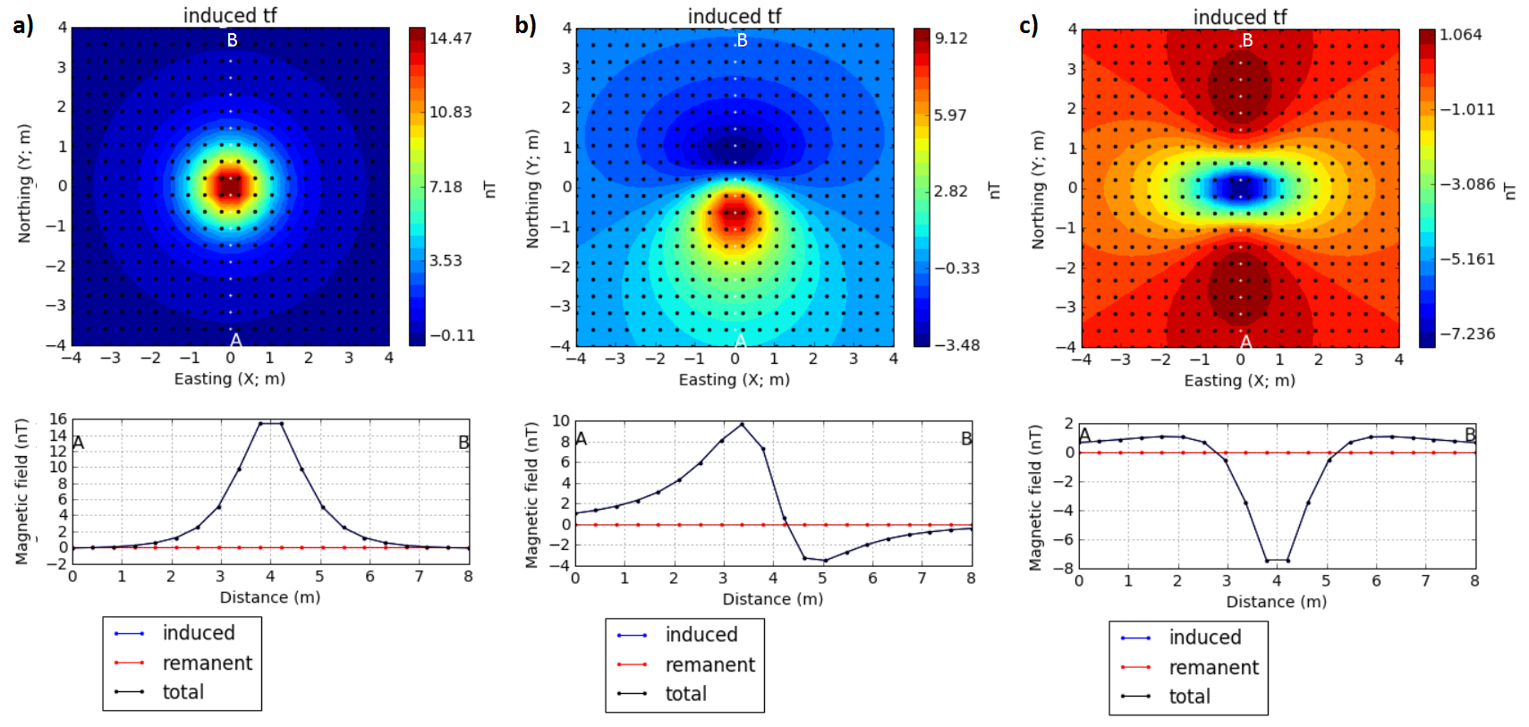
Fig. 42 Magnetic anomaly from a vertically orientation 2 m pole for differing inclinations of the Earth’s field: a) 90 \(\!\,^o\), b) 45 \(\!\,^o\) and c) 0 \(\!\,^o\).

To demonstrate the effectiveness of reduction to pole, let us consider a magnetic UXO survey (Fig. 43). On the left, we see the total magnetic field data collected at the survey site. Although anomalies indicate the presence of a number of potential targets, the location of each object relative to the anomaly it produces is inconsistent. However after completing a reduction to pole (right), the location of each potential targets becomes easily visible.

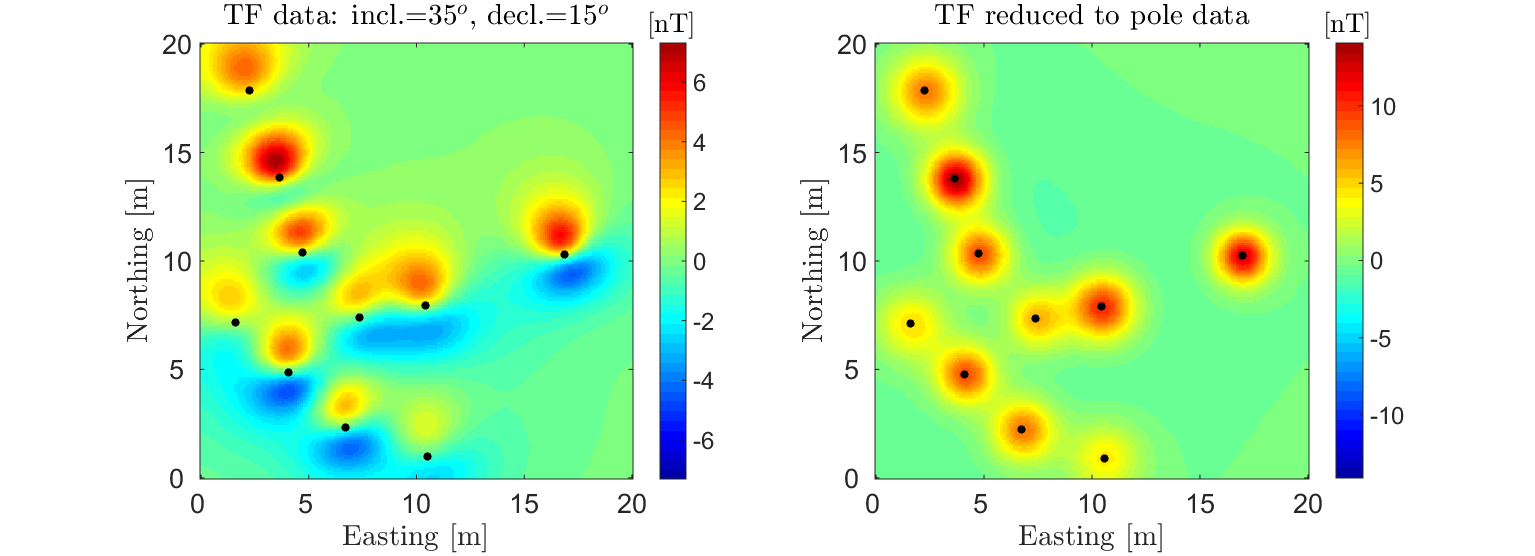
Fig. 43 Total field magnetic data over UXO before (left) reduction to pole and after (right) reduction to pole. The true location of each object is labeled by a black dot.