Interpretation
In this we focus on various techniques used to interpret the magnetic data. From an applied geoscientists standpoint, this is where most of the data integration and decision making steps are made. In some cases direct data interpretation can be used. In others, in particular when a 3D geologic interpretation is needed, an inversion is required. On this page, we discuss these techniques and illustrate common interpretation techniques on a mineral exploration example.
Direct Data Interpretation
We begin with direct data interpretation techniques. Informations about the sub-surface are inferred directly from the data, either through filtering methods or by analyzing the shape and amplitude of magnetic field anomalies.
Estimating Depth of Burial from Half-Width
For simple targets, a depth to the target can be estimated using the half- width. Most geologic setting are more complex and thus require more advanced interpretation.
As discussed in Basic Principles, in simple scenarios, the target of a survey can be approximated:
Consider a vertical inducing field (or alternatively, a data set that has been reduced to pole), and a profile line of data over a target located at the origin. The total field anomaly is expected to take a shape similar to that show in figure Fig. 44.
We define the half-width, \(x_{1/2}\), as the width of the anomaly at half its maximum (note that this is the anomaly, the background field has been removed).
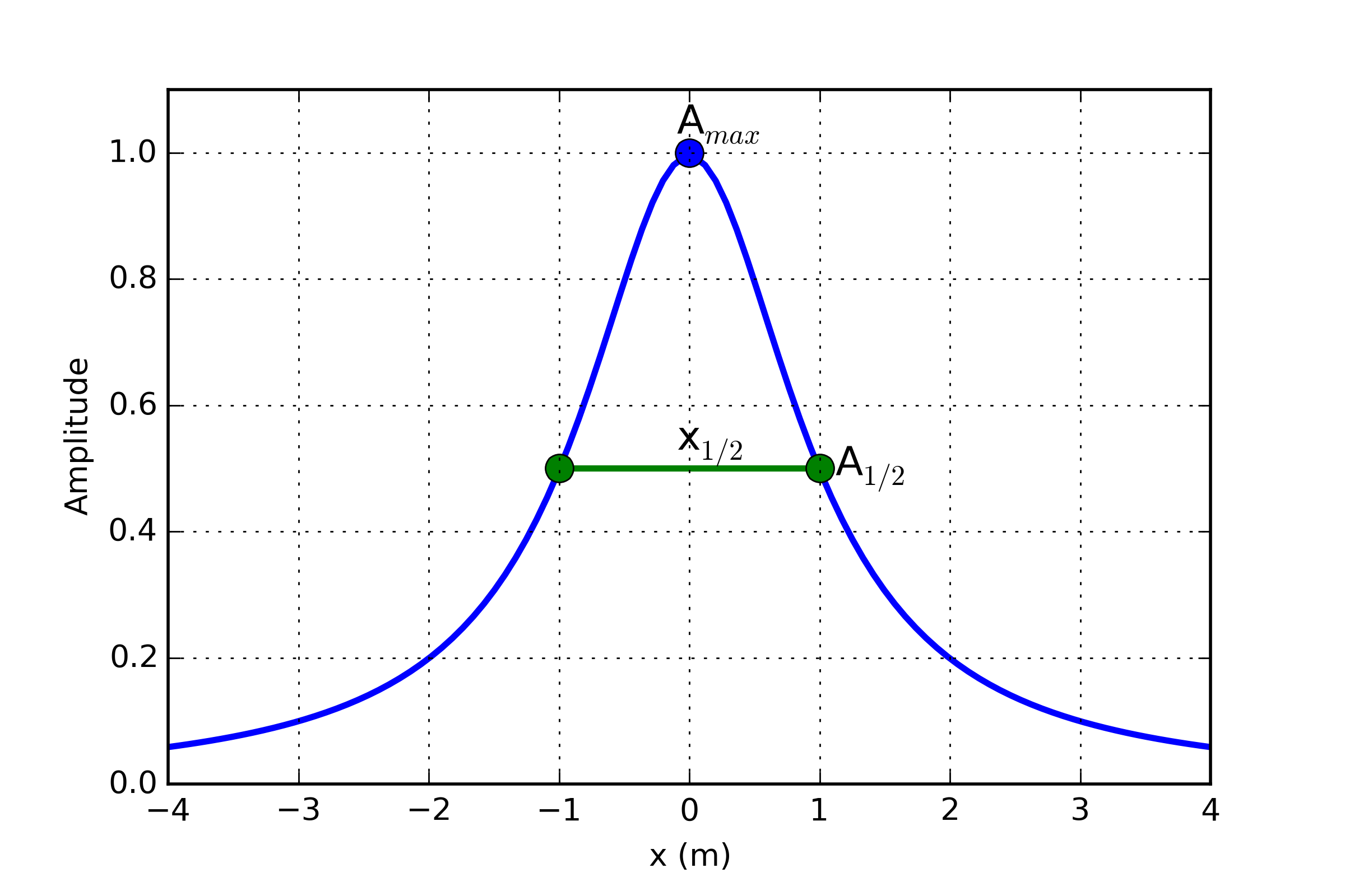
Fig. 44 Definition of half-width.
For a dipole target, the depth of burial(to the top of the target), \(z\), is approximately equal to the half-width
while for a monopole target, the depth of burial is
You can explore this concept further with the Jupyter Notebook app.
Derivative Maps
While the data itself can be informative, image filtering techniques are commonly used by industry to further highlight important features present in the data. These filters a generally done in the frequency_domain and require the data to be interpolated on a regular grid. Let \(M(x,y,0)\) be a grid of magnetic data taken at some reference elevation \(z=0\). Here are few filters applied to a simple 1x1x0.1 m block anomaly (Fig. 45):
Upward Continuation (UC): Magnetic data are synthetically moved vertically such that:
\[UC = M(x,y,\delta z)\]
Upward continuation is commonly used to remove the effects of very nearby (or shallow) susceptible material. High frequency information decays rapidly, leaving only the broad features. Downward continuation is also possible in order to accentuate the high frequency content, but comes at the risk of enhancing noise in the gridded data.
First vertical derivative (1VD): Quantifies the change in signal as a function of survey height.
\[1VD = \frac{\partial M}{\partial z}\]1VD maps are commonly used to enhance the shorter wavelength signal. Notice how well the linear features are defined compared to the Total Field profile.
Total horizontal derivative (THDR): Measures the lateral rate of change of the measured field.
\[THDR = \sqrt{\frac{\partial M}{\partial x}^2+\frac{\partial M}{\partial y}^2}\]This filter is most useful to highlight edges and delineate boundaries. Notice that the peak values occur over the edges of the block at -1 and 1 m.
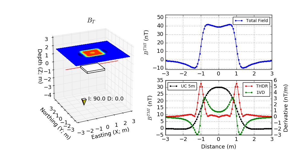
Fig. 45 Magnetics derivative based filters
Call for contributors
There are many other filters published in the literature. Please contact us if you would like to contribute to this page.
Tli Kwi Cho (TKC): A primer
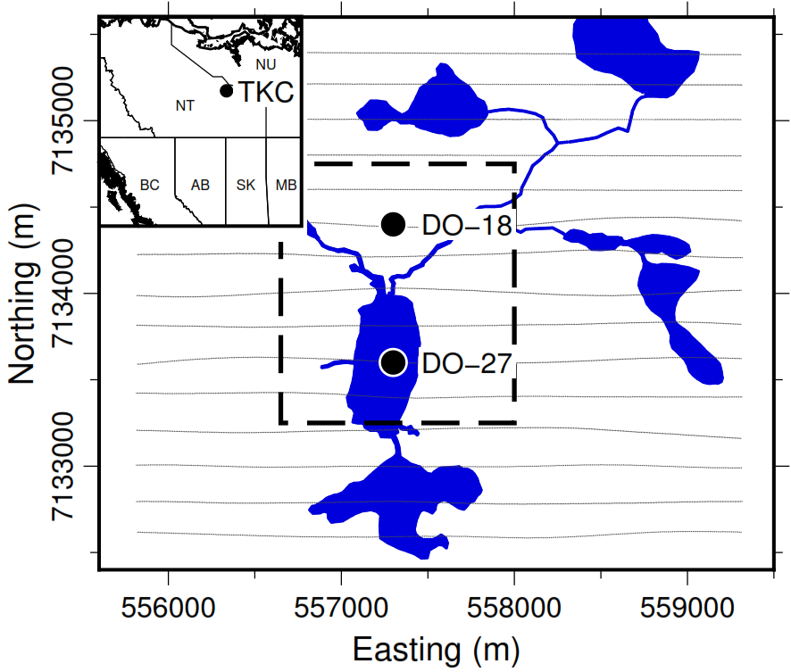
Fig. 46 Aquisition locations for TKC
We demonstrate the various interpretation techniques on a mineral exploration case study, the Tli Kwi Cho diamond deposit. Tli Kwi Cho (TKC) is a kimberlite complex in the Northwest Territories, Canada. The Northwest Territories have been surveyed extensively for diamondiferous kimberlites since the early 1980s. The Lac de Gras region has been particularly productive, and hosts two of the largest Canadian deposits: the Ekati and Diavik mines.
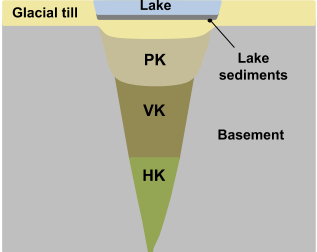
Fig. 47 Simplified sketch of expected TKC kimberlite deposit
A common geophysical fingerprint for a kimberlite pipe is a circular strong magnetic anomaly, with a gravitational low and an anomalous electromagnetic (EM) response. A generic model for kimberlite pipes found in the Lac de Gras region is presented in Fig. 47. The main rock types associated with kimberlites are summarized in Table 6.
Rock Type |
Description |
Susceptibility |
|---|---|---|
Pyroclastic Kimberlite (PK) |
Extrusive, violent, post-eruption |
Moderate-low |
Volcaniclastic Kimberlite (VK) |
Extrusive, fragmental, main body |
Moderate-low |
Hypabyssal Kimberlite (HK) |
Intrusive, igneous, coherent |
High |
Glacial till |
Sedimentary |
Low |
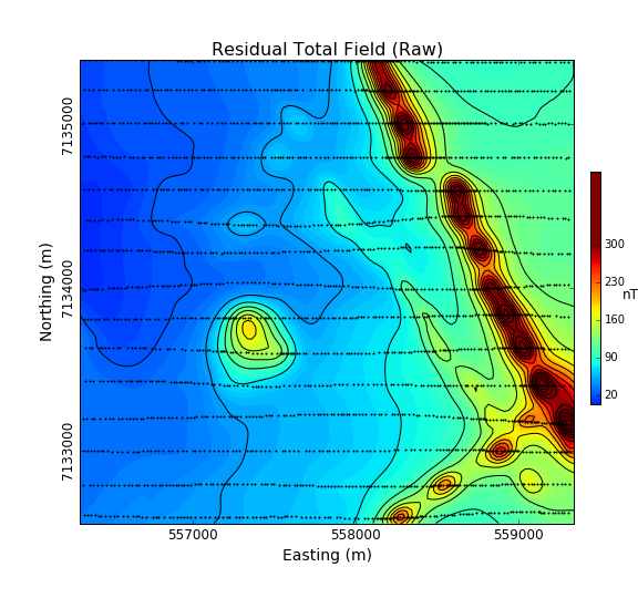
Fig. 48 Airborne magnetic data of TKC
The TKC kimberlite complex was identified from an airborne magnetic and frequency-domain electromagnetic DIGHEM survey in 1992 (Fig. 48). Geophysics had been used during the discovery phase of TKC, but little had been done to model the deposit prior to drilling. As we will later discover, the TKC deposit differ from the standard kimberlite model found in the region. Consequently, the geological model used to explain the deposit underwent several revisions over the following decades.
In this section, we will attempt to extract as much information as possible about the deposit strictly from the original airborne magnetic survey.
Data map
2D plots of magnetic data, often referred to as maps, can provide insight about the geologic units, contacts, and the horizontal location of structures. What is presented, and how it is presented can greatly alter interpretations obtained by visually analyzing the maps. Raw data are not usually presented directly. Choices of contour plotting parameters must be made; features not related to targets might be removed; and data or image enhancement processing might be employed. Here we introduce some aspects of these topics.
The first and simplest analysis can be done directly on the Total Field Anomaly data as shown below. The survey parameters are provided in Table 7.
Note: The highest values observed on the gridded magnetic map are strongly correlated with the survey line locations. This is strictly an interpolation bias and should be ignore during the interpretation process.
Inducing field |
\(Inc:\;83.8^\circ,\;Dec:\;25.4^\circ,\;Strength:\;60308\;nT\) |
Line spacing |
200 m |
Instrument |
Optical pump cesium vapor |
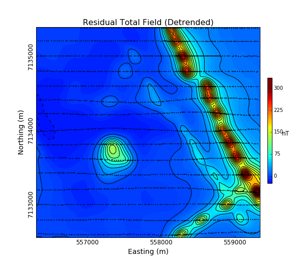
From the raw data, we notice a regional trend coming from the east of the survey area. In order to enhance the local anomalies, we first proceed with a regional trend removal. A \(1^{th}\) Order polynomial is subtracted from the raw data.
 |
Having isolated the local anomalies, we can now look at various filtering techniques as shown below:
 |
The derivative maps were useful in identifying at least two important features Fig. 49).
Two sets of elongated magnetic anomalies striking \(315^\circ\) N and \(45^\circ\) N. From the shape and strength of the magnetic field, they may correspond to intrusive dykes emplaced during separate events. From the THDR map, these dykes should be between 20 to 50 m in width.
Possible sinistral faulting post-intrusion striking at \(\approx 40^\circ\)
Two compact, near circular anomaly that could resemble a kimberlite pipes. These are features of interest in diamond exploration.
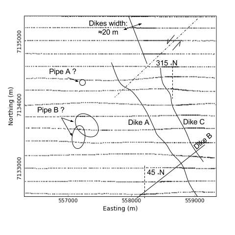
Fig. 49 Important features identified from the derivative maps
Parametric Simulation
From the data map, we have targeted two features of interest with different geometries: a narrow elongated anomaly and a compact body. In order to test these hypothesizes, we first attempt to approximate these magnetic features with simple parametric objects using the magnetic app.
Plate model
Fig. 50 compares the observed and simulated magnetic data across an elongated magnetic anomaly. The parameter used for the plate model are presented in Table 8. This result seems to confirm the presence of thin, shallow dipping magnetic dykes.Turns out that these dykes are part of the Mackenzie dyke swarm that runs through out the Lac de Gras region. These intrusive dykes are related to major tectonic events, and although interesting scientifically, they are of little interest in diamond exploration.
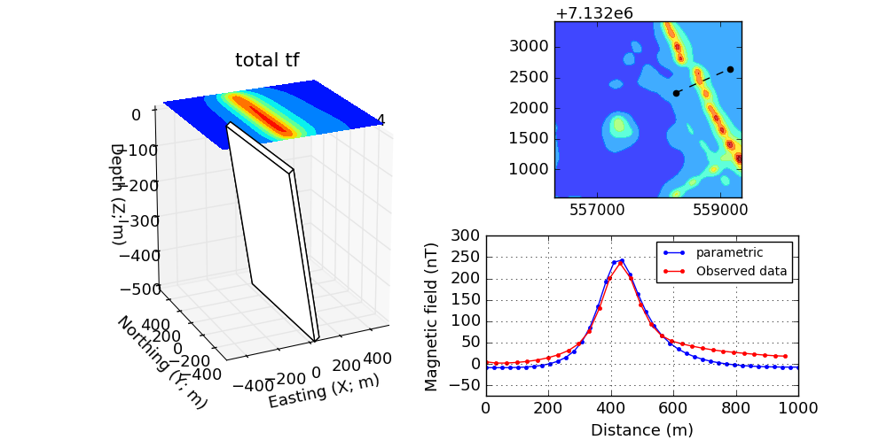
Fig. 50 Parametric dyke model of TKC area
Dimensions |
50 x 800 x 500 m |
Dip |
\(20^\circ\) |
Susceptibility |
0.1 SI |
Pipe model
Second, we look at the compact, near circular magnetic anomaly in the center of the survey area. This feature may be of interest as it resemble the typical signature of a kimberlite pipe. Fig. 51 compares the magnetic data over the compact anomaly and the parametric pipe model (Table 8). This result seems to confirm the presence of a compact magnetic block SE dipping. The shape of the anomaly is surprisingly different than the expected shape of a vertical pipe. This result requires additional work for validation, hence the need to invert the data.
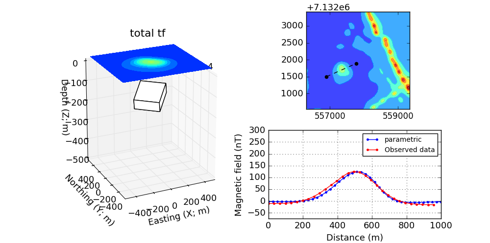
Fig. 51 Circular pipe model of the TKC area
Dimensions |
300 x 200 x 50 m |
Dip |
\(20^\circ\) |
Susceptibility |
0.05 SI |
Inversion
The parametric forward simulation was helpful in understanding the shape and susceptibility contrast associated with the main magnetic anomalies. Modeling the Earth with simple parametric objects rapidly becomes prohibitive however for large and complicated susceptibility distributions. For this reason, we must adopt a more mathematical approach.
The inverse problem is illustrated in Fig. 52. Similar to a medical imaging problem, the goal is to recover a 3D representation of the Earth from the magnetic data. Several commercial and open-source algorithms are available to solve the inverse problem. We here used the SimPEG open-source package. We present the various input parameters required for the inversion.
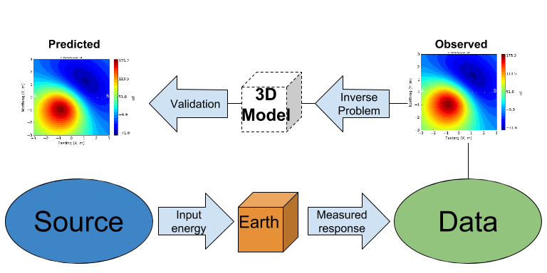
Fig. 52 Conceptual inverse problem
Inverse Problem
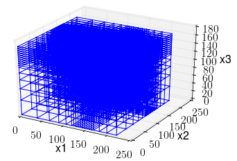
Fig. 53 Mesh used to discretize the subsurface for inversion
In its simplest form, the inverse problem attempts to image the Earth from the observed data. To do this, we need to approximate the continuous Earth with a set of discrete parameters that a computer can understand. A picture taken with a digital camera is a great analogy. The quality of the picture largely depends on the resolution of the camera, or the number of pixels used to capture the image. The higher the resolution, the larger the file size. Similarly for 3D inversion, we need to choose an appropriate mesh resolution to capture the right level of details, without getting too large for a computer to handle it. The chosen mesh parameters for this problem are shown in Table 10.
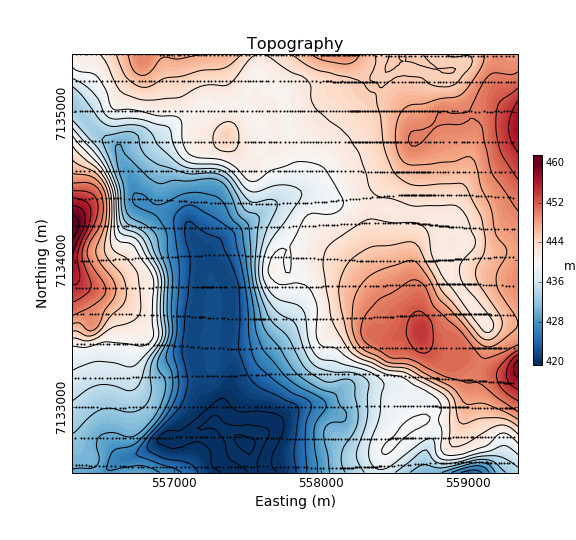
Fig. 54 Topography of the TKC area
Secondly, we need a topographic surface that defines the relative distance between the observation point and the discrete Earth. A Digital Elevation Model (DEM) is downloaded from the NRCan Geogratis website as shown in Fig. 54.
Cell size |
25 x 25 x 25 m |
Number of cells (X, Y, Z) |
120 x 130 x 35 = 546,000 cells |
Number of data |
1092 |
Data uncertainties |
10 nT |
3D Solution
From the inversion algorithm, we recover a 3D model of magnetic susceptibility. We note the following features:
The inversion successfully recovered thin dipping planes similar to our parametric model. Despite getting smooth and broad at depth, the vertical length of these magnetic planes appear to extend from the surface down to over 500 m (Fig. 55 ).
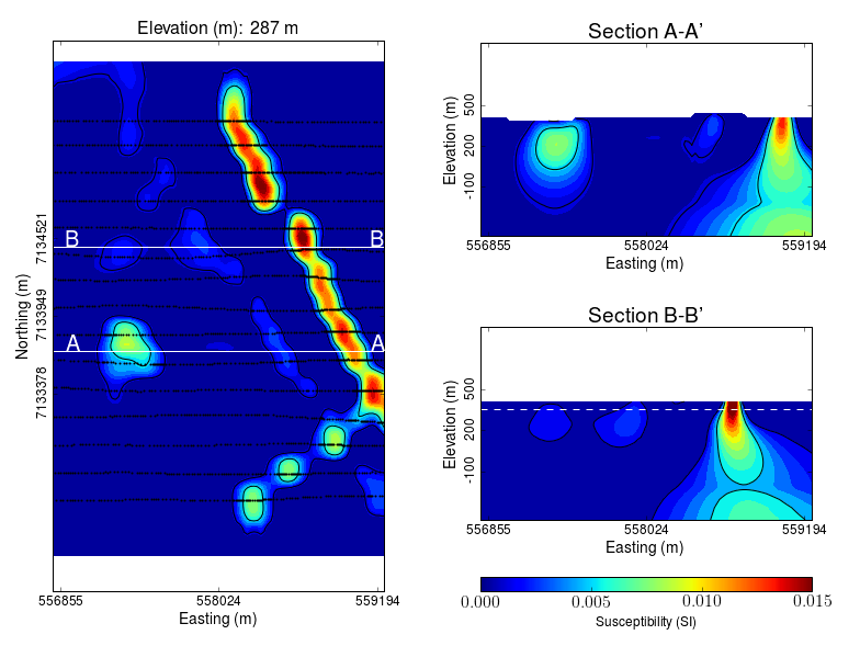
Fig. 55 Inverted TKC susceptibility model
Two nearly vertical compact bodies are imaged west of the magnetic dykes (Fig. 56). Susceptibility values vary greatly between the two anomalies. The largest (South) anomaly seems to dip slightly toward SW has predicted by our parametric model and appears deeper than the northern anomaly.
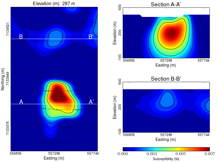
Fig. 56 Vertically compact bodies identified with inversion
Validation
A key component to asses the validity of our 3D model is to verify that the given solution honors the data. The figures below compares the true and predicted magnetic data. The residual map confirms that our model captures most of the signal contained in the airborne data set.
 |