Chargeability
Chargeability is a physical property related to conductivity. As we learned previously, ionic charges within a rock’s pore water begin to move under the influence of an electric field, resulting in electrical current. However, some of the pore ions do not move uninhibited through the rock and begin to accumulate at impermeable boundaries. This build-up of ionic charges is commonly referred to as induced polarization (IP), as it is responsible for generating electric dipole moments within the rock. We use chargeability to characterize the formation and strength of the induced polarization within a rock, under the influence of an electric field.
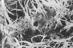
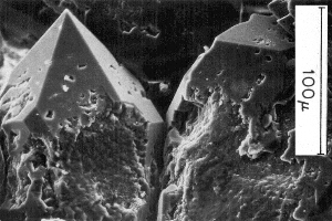
The physical explanation for causes of chargeabilty are complex and not completely understood. Certainly the effects are dependent upon the microscopic nature the material and specifically upon the surface to volume ratio of pore material and the types of fluids in the rock. The two images below offer some insight into the complexity.
Despite the complexity are two primary phenomenological mechanisms which are insightful in characterizing the chargeable behaviour of rocks: membrane polarization and electrode polarization.
Membrane Polarization
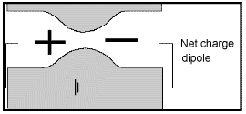
Membrane polarization occurs when the pore space narrows to a within several ion widths.
Because ionic charges cannot be forced through the pore throat, they accumulate on either side when an electric field is applied; with positive charges accumulating on one side of the pore throat and negative charges accumulating on the other. The accumulation of charges eventually stops because the electric fields from the blocked charges becomes large enough that it prevents other ions of the same sign from joining the group.
The net separation of positive and negative charges across narrow pore spaces generates a set of electric dipole moments which is ultimately responsible for the voltages measured in induced polarization survey.
Electrode Polarization
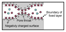
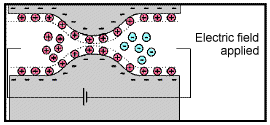
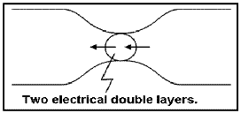
Electrode polarization occurs when the pore space is blocked by metallic particles. When an electric field is applied, the metallic particles become electrically charged and attract nearby ions.
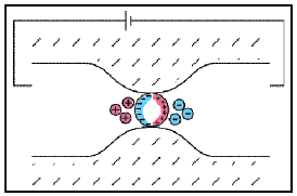
The attraction of the ions to the surface forms a primary layer of fixed ionic charges, followed by a secondary diffuse layer of opposing charges. This is known as an electric double layer.
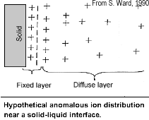
Each electric double layer results in an electric dipole moment which contributes towards the induced polarization within the rock.
Effects of IP on Geophysical Measurements
To demonstrate the effects of induced polarization on geophysical measurements, consider a specific example where a current generator, hooked to the ground as in a DC survey, is turned on. At some location, the electric potential (\(V\)) is measured. In non-chargeable rocks, an instantaneous increase in the measured potential occurs when the source is switched on. When the source is switched off, the current through the Earth returns immediately to zero and so is the measured potential. This is illustrated in the figure below.
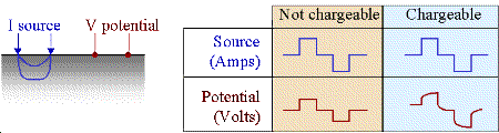
If the ground is chargeable, there will also be an instantaneous jump in the measured potential when the source is switched on; we denote as \(V_\sigma\). However, the subsequent build-up of ionic charges during the on-time results in a corresponding increase in the measured potential; which is sometimes referred to as the over-voltage. Eventually, the build-up of ionic charges reaches saturation, resulting in a final measured potential (\(V_m\)). In general, the measured potential after the source is switched (\(V_{on}\)) can be expressed as:
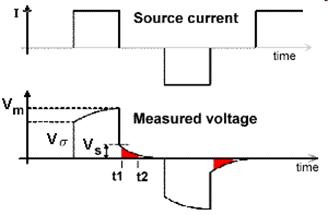
where \(V_s\) is the amplitude of the over-voltage and \(\tau\) is a constant which determines the rate at which the induced polarization forms.
When the source is switched off, there is an instantaneous drop in the measured potential equal to \(V_\sigma\). Subsequently, the accumulated charges begin to diffuse, resulting in a measured potential which decays according to:
This decaying off-time potential is commonly called the discharge curve. We use the discharge curve to characterize the chargeable properties of the Earth.
Definitions for Chargeability
It is convenient to consider “chargeabilty” as an independent physical property but in reality it is an integral component of the electrical conductivity. It describes how the conductivity changes with frequency. If \(\sigma_0\) denotes the conductivity at zero frequency and if \(\sigma_\infty\) is the conductivity at infinite frequency then the chargeability is
This is a dimensionless number varying between 0 < \(\eta\) < 1. It is often referred to as the intrinsic chargeability. The above definition is equivalent to defining the intrinsic chargeability as the ratio between the amplitude of the over-voltage (\(V_s\)) and the DC voltage (\(V_m\)):
The intrinsic chargeability for materials is rarely provided in tables. Rather, numbers based upon laboratory measurements of some characteristic of the induced polarization response is provided. Those measurements can be in time or frequency and the units of the “chargeability” are inherited from the data. We outline below:
Two types of time domain data
The following is a definition of chargeability but it is not possible to measure it exactly in the field. The figure to the right shows voltage measured when the transmitter is first turned on and then turned off some time later. Using parameters from this figure, one definition of chargeability is \(M = V_S / V_P\) where \(V_S\) and \(V_P\) are the steady state and “secondary” potentials, respectively.
The leading edge potential \(V_{\sigma}\) is what would be measured in the absence of chargeability. This potential would yield the ground’s resistivity.
The steady state, \(V_P\) (with a subscript m in the figure above), often referred to as the primary potential, is the combined effect of current flowing in the ground and charges built up under the influence of the imposed electric field.
The secondary potential is entirely due to the charge imbalance resulting from the build-up of charge.
Using this form, chargeability \(M\) will be \(0 ≤ M < 1\). If \(M = 0\) the measured potential will follow the input current waveform exactly with no charging or discharging involved, as shown in the first column of the figure above.
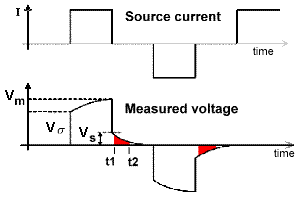
The most commonly measured form of time domain IP is the normalized area under the decay curve. It can be represented by the following equation, using parameters specified in the adjacent figure. The decaying potential that follows \(V_s\) is written as \(V_s (t)\).
Chargeability, \(M\), is essentially the red area under the decay curve, normalized by the source voltage.
\[M = \frac{1}{V_P} \int \! V_S(t) \, \mathrm{d}t\]
Integrated Chargeability
The integrated chargeability (\(M\)) characterizes the quantity of potential energy stored within a chargeable rock due to the accumulation of ionic charges. The integrated chargeability is defined as the area under the discharge curve normalized by the DC voltage (\(V_m\)):
Numerical values for the integrated chargeability are typically given in ms.
Two types of frequency domain data
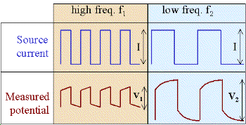
An oscillating source current can be employed to observe chargeability. The measurements are often still referred to as “DC resistivity” because the frequencies are relatively low. The resulting data will include (i) a “DC resistivity” based upon the voltages measured with the lowest source frequency, and (ii) a chargeability based upon the measurements explained next. Two methods of measuring chargeability in the frequency domain are described below.
If the amplitude of the potential is measured at two frequencies, a measure of chargeability is acquired, and it can be expressed as units of “percent frequency effect” or PFE. Since the ground has less time to respond at higher frequencies, the signal is expected to be smaller at the higher frequency. Expressions for PFE are shown in the equations below. The data used in this calculation are illustrated in the figure below. Recall that \(\rho_a= K \mid V \mid / I\) , where \(K\) is the geometric factor based upon electrode geometry (see the Geophysical surveys chapter, “DC resistivity” section), \(V\) is the measured potential, and \(I\) is the source current.
Alternatively:
If the voltage version is used, the Frequency Effect (FE) can easily be converted to a percent frequency effect by multiplying by 100.
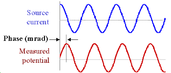
Data with units of phase are gathered by transmitting a sinusoidal source current. Then the phase difference between this source and measured potentials is recorded as a measure of chargeability. Units are usually milliradians. The following figure illustrates:
Relating the four types of data
The different IP responses all result from the build up of polarizing charges, but they do not produce the same numbers. In fact, the units of the various measurements are different. Nevertheless, the following approximate rule of thumb allows conversion between the different data sets:
A chargeability of \(M = 0.1\) is
10 PFE
70 mrad
70 msec
Chargeability Measurements
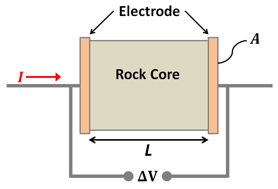
For integrated and intrinsic chargeability measurements, a core sample is taken from the rock. The core sample is then placed in a sample holder between two copper/graphite electrodes where it acts as an impedence element for a circuit.
Integrated Chargeability Measurements
For integrated chargeability measurements, a source is used to drive direct current (\(I\)) through the rock core. During the on-time, the voltage (\(V_m\)) is measured across the sample. Next, the source is switched off. During the off-time, the potential across the rock is measured as it decays. The off-time measurements are used to define the discharge curve for the sample, which is then used to obtain the integrated chargeability according to:
For practical measurements, we do not integrate over the entire discharge curve. Instead, a finite interval of integration is chosen. For example, the Newmont standard chargeability integrates from t = 0.15 s to 1.1 s.
Intrinsic Chargeability Measurements
Intrinsic chargeability measurements are very similar to conductivity/resistivity measurements. In this case, the source is used to drive alternating current (\(I\)) through the core sample. By measuring the voltage drop (\(\Delta V\)) accross the length of the sample, Ohm’s law can be used to determine the circuit impedence (\(Z\)) caused by the rock:
In chargeable rocks, the measured voltage drop depends on the frequency of the alternating current. So in order to characterize the resistive properties of the rock, we need to determine the impedence over a spectrum of frequencies.
The resistivity of the sample at each frequency can be obtained from the impedence, the length of the core (\(L\)) and its cross-sectional area (\(A\)) using Pouillet’s law:
In order to characterize the rock’s chargeable properties, we fit the experimentally acquired resistivity values to a mathematical model (illstrated below). A well-established model for explaining the resistivities of chargeable rocks is the Cole-Cole model:
where \(\rho_0\) is the DC resistivity and \(\eta\) is the intrinsic chargeability. Parameters \(\tau\) and \(C\) define the rate at which ionic charges accumulate when an electric field is applied.
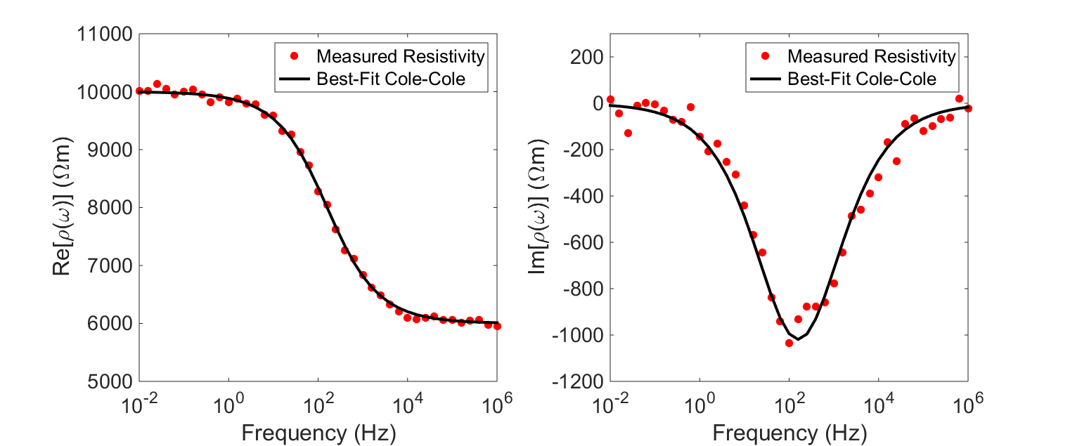
Assuming \(C=1\), \(\tau\) defines the exponential decay in voltage during the off-time measurements (see earlier). The conductivity of the rock can be obtained by taking the reciprocal of the complex resistivity:
Additionally, Ohm’s law still applies for chargeable rocks. Thus:
Chargeabilities of Common Rocks
Tables (from Telford et al, 1976) provide a very general guide to the integrated chargeabilities of materials. Because different intervals of integration \([t_1,t_2]\) are used for each table, chargeability values cannot be compared between tables. However, we can infer several things from these tables:
The individual properties of rocks results in a variation in chargeability (click here for table).
Chargeability increases as the % abundance of sulphide minerals increases (click here for table).
Highly porous rocks such as extrusive volcanics and sandstones are more chargeable than hard rocks such as granites and limestones (click here for table).
The type of ore-mineralization impacts the chargeability of rocks to varying degrees (click here for table).
Factors Impacting Chargeability
Sulphide Mineralization:
As we discussed earlier, electrode polarization occurs when the pore path is blocked by metallic particles. A major source of these metallic particles is sulphide mineralization. As the abundance of sulphide minerals within a rock increases, so does the electrode polarization. Therefore, highly mineralized rock tend to be very chargeable.
Clays:
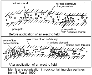
Clays have a tendancy to partially block the path which ions take through the rock’s pore water. Upon application of an electric potential, positive charge carriers pass easily, while negative carriers accumulate. This results in an “ion-selective” membrane polarization. Clays represent a dominant source of induced polarization in unmineralized sedimentary rocks.
A surplus of both cations and anions occurs at one end of the membrane, while a deficiency occurs at the other end. The reduction of mobility is most obvious at frequencies slower than the diffusion time of ions between adjacent membrane zones; i.e. slower than around 0.1 Hz. Conductivity increases at higher frequencies.
Pore-Water Salinity:
The induced polarization within a rock depends on having a mechanism for accumulating ionic charges. It also depends on the salinity of the pore water; i.e. the concentration of ions within the pore water. As the pore-water salinity increases, so does the capacity of the rock to support a build-up of ionic charges. This results in an increases chargeability for the rock.
Tortuosity:
Tortuosity defines the connectivity and complexity of a rock’s pore-space network. As the tortuosity of the rock’s pore-space increases, it becomes more difficult for ionic charges to move through the rock. As a result, and increases abundance of ionic charges will accumulate within the rock when it is subjected to an electric field. Thus, the chargeability of a rock increases and its tortuosity increases.