Interpretation

Forward Modeling

Essential equations

We start by considering a theoretical form of time-domain IP data. Recall that if a square current signal is injected into the ground, the potential recorded over chargeable ground will exhibit a delayed response caused by the charging and discharging of the ground. There are three potentials that can be defined on this measured voltage waveform, as shown on the adjacent figure. The theoretical IP datum is defined as the ratio of the secondary voltage measured immediately upon shutting off the current source to the primary voltage measured after the signal has stabilized while the current is still on.

\[d= \frac{V_s}{V_P} = \frac{V_P - V _ {\sigma}}{V_P} = \frac{F_{DC}[\sigma (1 - m)] - F_{DC}[\sigma]}{F_{DC}[\sigma (1 - m)] }\]

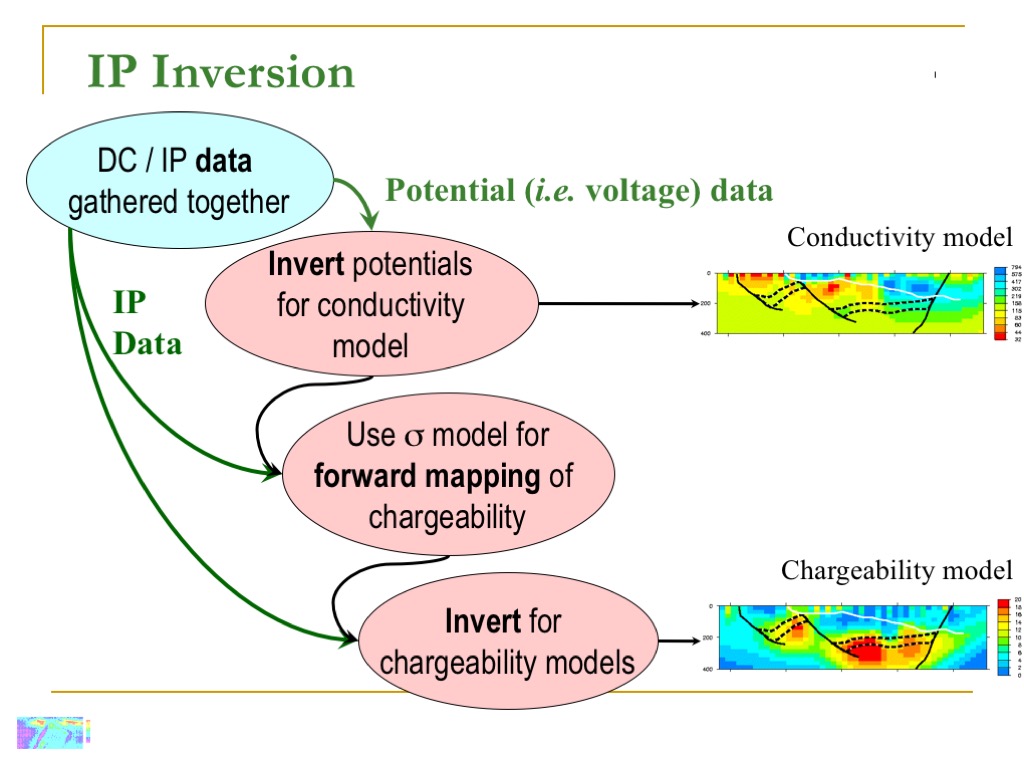
The right hand side of this equation is showing that each potential can be found using a DC resistivity forward modeling calculation using the conductivity of the region involved, and that conductivity is modified by chargeability, \(m\). This is based upon the original definition of chargeablity suggested by Seigel, 1959.

This equation turns out to be non-linear. It can, however, be approximated as linear for small values of \(m\), which is usually true since in practice \(m < 0.2\). Therefore, forward modeling of chargeability data can be done using the following formulation:

\[d_i = \sum\limits_{j=1}^n J_{ij} m_j \quad \textrm{;} \quad J_{ij} = - \frac{\partial \ln (V_i)}{\partial \ln ( \sigma_j)}\]

The matrix form for this equation is \(Jm = d\), where \(J\) is an N x M sensitivity matrix (N is the number of data points and M is the number of cells in a rectangular discretization grid), and the \(J_{ij}\) are sensitivities for the DC resistivity problem. So in order to model (and invert) IP data for interpretation, we need to solve the DC problem first.

Finally, if “small” chargeabilities are assumed, the linear relationship means measured data and chargeabilities recovered by inversion have the same units. Therefore, all four types of IP data can be approximated by \(Jm = d\). This means that the common types of IP data (time domain, phase, or PFE) can be employed as input to inversion routines without change.

These points are made in Oldenburg and Li, 1994.

Inversion of IP data

Inversion of IP data is related to the inversion of DC data (see Interpretation). Concepts such as Depth of Investigation still hold in the IP case.

Inversion of IP data requires a conductivity model obtained by inverted the DC data, as the sensitivity of an IP survey depends on the electrical conductivity distribution.

References

1. Siegel. H.O., 1959, “Mathematical formulation and type curves for induced polarization”, Geophysics, 38, 49-60.

2. Oldenburg, D.W. and Y. Li, 1994, “Inversion of induced polarization data”, Geophysics, 59, 1327-1341.