Gravity data: acquisition and reduction
Instrumentation: part I
Modern portable land-based instruments include automated leveling, data recording, and logging, but essentially their sensors are based upon variations of a mass on a spring. If the force on a spring is to be measured accurately to tell us geologically useful information about gravity, then changes in spring length, \(ds\), must be measured with a precision of 1:109. Therefore, some form of “amplification” is required. A complete discussion of instruments is beyond the scope of these notes, but some of the characteristics of the most common instruments are listed here.
Conventional instruments available until the 1990’s used LaCoste and Romberg or Worden methods of enhancing the effects of spring length changes. These instruments are still useful and accurate, though systems are available that are easier and quicker to use. See below.
A “zero length” spring is used, since they have tension proportional to absolute length, rather than to extension from unstressed length.
They operate as “null” instruments. A second spring is used to restore the mass beam to the zero position, and a micrometer dial reads off the force required. A calibration constant converts the dial reading to units of \(g\).
These are mechanical instruments subject to drift, temperature effects, and shock. Use of quartz components, temperature compensation, thermos-flask cases, shipping clamps, etc. help stabilize the instruments.
The figure to the right shows a diagramatic cross-section of the “works” inside a Worden gravimeter, from Exploration Geophysics of the Shallow Subsurface, by H.R. Burger, Prentice Hall.
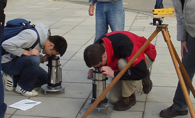
The figure below shows students using two Worden gravimeters in a field exercise, along with a simple laser leveling instrument from a hardware store to obtain relative elevations with roughly 1 cm accuracy.
Instrumentation: part II
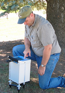
Modern instruments use similar mechanisms, but they incorporate automatic leveling, computer driven recording, and other convenience features.
There are also several organizations supplying instruments and services for marine and airborne surveys, and for measuring gravity gradients, but these advanced topics are beyond the scope of this introduction, except for the comments on the associated page that discusses gravity gradients.
Field procedures
The following points provide an outline for how data are acquired for common ground-based surveys.
Calibration: A constant is used to convert dial reading to the proper units (milliGal). This can be set by the manufacturer, or by recording at a known site.
Setting the range: Only relative gravitational changes can be recorded unless measurements are tied to a benchmark with a known value of \(g\). The dynamic range of an instrument may be between 10,000 and 70,000 mGal, and the instrument’s range may have to be set for a new site after the instrument has been transported.
Shake-down: Gentle tapping on the base may be required to stabilize the movement (especially after resetting the range).
Leveling the instrument: Leveling is critical. Ensure the platform is stable and not drifting. Be aware of ground motion, vehicles, trees, tele- and micro-seismics, etc.
Readings: Ideally, several readings should be made by a single operator, each one involving a separate leveling. To avoid dial “whiplash,” view comfortably from a consistent angle, and adjust the instrument for its null reading, using the exact same physical procedure every time.
- Survey procedures:
Station spacing depends on anomaly size; avoid spatial aliasing, unless anomaly detection (as opposed to anomaly characterization) is the only goal.
Most surveys involve measurement of relative values. A base station is chosen and re-occupied often enough (every couple of hours) to characterize instrument drift. Results are generated relative to it.
Surveys requiring absolute values of Earth’s gravitational field can be done with relative instruments by tying measurements into a station that is part of the IGSN (International Gravity Standardization Network).
For accuracy of 1 gu (0.1 mGal), read gravity to 0.1 gu, latitude to 10 m, elevation to 1 cm.
The following are some comments on positioning for gravity surveying:
3.3 cm elevation error results in 0.01 mGal measurement error, which is the accuracy of many instruments.
Centimeter accuracy in elevation is possible with realtime differential GPS, but it is not necessarily easy.
Terrain corrections are hard to get accurate to better than 0.2 mGal using conventional methods because of line-of-site limitation for “inner zone” corrections. However, digital terrain data can contribute significantly to improving final results.
Data reduction
The goal of data reduction is to remove the known effects caused by predictable features that are not part of the “target.” The remaining anomaly is then interpreted in terms of sub-surface variations in density. Each known effect is removed from observed data. First the various “corrections” are described, and then the presentation options are listed.
Corrections
The adjacent figure shows the effects of each correction for a short line surveyed in Vancouver, BC. Raw data after correcting for drift, and each of the correction factors are shown. Final interpretations would normally be made from the Bouguer anomaly graph (red).
Latitude correction: The earth’s poles are closer to the center of the equator than is the equator. However, there is more mass under the equator and there is an opposing centrifugal acceleration at the equator. The net effect is that gravity is greater at the poles than the equator.
For values relative to a base station, gravity increases as you move north, so subtract \(0.811sin(2a)\) mGal/km as you move north from the base station. (The \(a\) is latitude).
The maximum correction values will be 0.008 mGal / 10 cm, which occurs at \(a=45°\).
Free-air correction (elevation): Applying 0.3086 h mGal (h in meters) accounts for the \(1/r^2\) dependence. Measurements at higher elevations will be smaller; therefore, add the correction for higher elevations.
Bouguer correction: This corrects the free-air value to account for material between the reference and measurement elevations. If you are further above the reference, there is more material (effect is greater), so subtract \(0.04191 h× d\) mGal (\(h\) in metres, \(d\) in g/cc) from the reading. The derivation involves determining the effect of a point, then integrating for a line, then again for a sheet, and finally for a slab.
In the equation for the Bouguer correction, density, d, must be estimated; this can be done if the material is known, or by using a “crustal” value of 2.67 g/cc. Alternatively, trial and error can be used to find the density that causes the data to least reflect the patterns of topography.
Question: The Bouguer correction is always subtracted. What situation causes the value to be positive, and what causes the value to be negative?
Topography, or terrain correction: This correction accounts for extra mass above (hills, etc.), or deficit of mass (valleys, etc.) below a reading’s elevation. By hand, this involves the use of a “Hammer chart” and tables, although the process is not very accurate. More modern methods require software that makes use of digital terrain models (DTM) available from government or third party sources.
Earth-tides: Tidal variations are slow enough that, for most surveys, they are handled as part of the drift correction; i.e. by recording values at a base station every few hours.
Eötvös correction: This is the correction necessary if the instrument is on a moving platform, such as a ship or aircraft. It accounts for centrifugal acceleration due to motion on the rotating earth. The relation is
where:math:V is speed in knots, \(\alpha\) is heading, and \(\phi\) is latitude. At mid-latitudes, it is about 7.5 mGal for 1 knot of E-W motion.
Data presentation options
Just what is plotted as a profile or map depends upon which corrections are applied. Commonly plotted quantities are as follows:
Free air anomaly: In local surveys, we use a base station value for \(g_t\). The free air anomaly is required for some modeling programs when terrain is accounted for exactly.
Bouger anomaly: This includes the free air anomaly, plus the Bouguer correction, and topographic corrections. Some authors do not include topographic corrections in the Bouguer anomaly; all you can do is check carefully each time.
Removal of regional effects: It is important to de-emphasize effects of deep or large masses that are not of interest. Regional removal is often done by fitting a polynomial line or surface to the data. To first order a straight line is usually okay for small surveys. Graphical (visual) fitting is not rigorous, but often works well. Click this Gravity example for a brief discussion of an example of trend removal applied to a re-examination of an older gravity survey over a petroleum reservoir in Oklahoma.
Plot residual: What is left after removing the regional trend.
Note that 2D data sets usually require gridding, which is a whole story unto itself.