Survey

Dual Loop Systems

EM-31

Loop-loop system mounted on a 4 meter boom. The transmitting coil operates at a frequency of 9.8 kHz and the receiving coil is located 3.66 meters from the transmitter. The instrument measures both the in-phase and quadrature fields. The in-phase component is diagnostic of high conductivity bodies (metal pipes, drums, etc.) and the quadrature component can be converted into an apparent conductivity which is read out in mS/m. Such readings arc valid only if the ground is laterally uniform on a scale length equal to the source-receiver separation and that \(s << \delta\). The instrument and coils can be rotated by 90° so that loops are vertical. This provides data estimating the conductivities and thickness. The effective depth of exploration is about 6 meters for the vertical dipole mode and about 3 meters for the horizontal dipole mode. Data can be acquired with the device held at hip level or it can be put on the ground.

EM-34

This uses two vertical or horizontal coplanar coils that are not attached to each other. The coils and analysis system are designed so that different coil separations operate at different frequencies:

1. 10 meters at 6.4 kHz

2. 20 meters at 1.6 kHz

3. 40 meters at 0.4 kHz

This allows greater penetration into the ground and hence is used to delineate vertical geologic anomalies and for groundwater exploration in fractured, faulted and weathered bedrock zones.

Depth of Investigation

A maximum depth of investigation is provided by the skin depth rule, however for controlled source surveys we also need to take into account the source and receiver geometry. This generally reduces the depth of penetration. A rule of thumb for loop-loop systems is that the depth of penetration is about twice the separation of the source and receiver, but this is very approximate and is easily violated. Also, a necessary condition for this to happen is that the source/receiver separation \(s << \delta\) (coil separation is less than the skin depth).

If we are attempting to find a conducting target then the ability to see the target depends upon the coil orientation and coil separation. It must also take into account the fact that the:

1. primary field is attenuated before it reaches the target

2. the secondary fields are attenuated as they travel from the target to the receiver.

Apparent Conductivity from the Quadrature Component

If the spacing \(s\) between the coils is much less than the skin depth, that is, \(s << \delta\) then the ratio of secondary to primary field is approximately

\[\frac{H_s}{H_p} \simeq i\frac{\omega \mu_0 \sigma s^2}{4}\]

where \(i\) is the imaginary unit. The response is purely imaginary, that is, it is found in the quadrature component of the data. The constant conductivity which gives rise to the observed response can be found from the above formula. It is referred to as the apparent conductivity \(\sigma_a\):

\[\sigma_a = \frac{4}{\omega \mu_0 s^2} \mathrm{Im}\left\{\frac{H_s}{H_p} \right\},\]

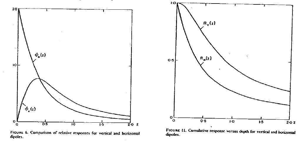
where \(\mathrm{Im}\left\{\frac{H_s}{H_p} \right\}\) is the imaginary part of the secondary field to primary field ratio. Further insight about the apparent conductivity is obtained by incorporating the response curves \(\phi_V(z)\) and \(\phi_H(z)\). We have

\[\begin{split}\sigma_a &= \int_{0}^{\infty} \phi_V (z) \sigma (z) dz \\[0.8em] \sigma_a &= \int_{0}^{\infty} \phi_H (z) \sigma (z) dz\end{split}\]

respectively for the vertical and horizontal dipoles.

Relative Response Function

The justification for the above statement is based upon the following. Consider a homogeneous halfspace on the surface of which is located a horizontal coplanar coil (HCP) system (e.g. EM31) or a vertical coplanar (VCP) system (EM34). Let the depth \(z\) in the earth be normalized by the coil spacing \(s\). (True depth in meters is \(zs\).) The time varying fields in the transmitting coils will induce eddy currents in the earth. For a homogeneous earth, these currents flow in horizontal planes. This is true even for the vertically oriented coils. It is possible to calculate the contribution to the secondary field as measured from the surface from any thin layer of thickness \(dz\) at some depth \(z\). Let \(\phi_V(z)\) denote this contribution from the vertical magnetic dipole source and receiver. The subscript \(V\) denotes that the magnetic fields are vertical. A horizontal loop of current acts like a vertical magnetic dipole. A plot of this function is shown below:

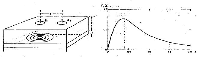
Fig. 145 Relative response versus depth for vertical dipoles. \(\phi_V(z)\) is the relative contribution to \(H_s\). from material in a thin layer dz located at (normalized) depth \(z\).

Note that the vertical magnetic dipole has zero sensitivity at the surface, has a maximum at about \(z = 0.4\) and is substantially diminished by \(z = 2.0\). It is this type of diagram which says that the maximum depth of investigation is limited to about twice the coil separation. This rule of thumb however is valid only when the coil separation is much less than the skin depth.

The response function from the horizontal magnetic is very different. Let \(\phi_H (z)\) denote the relative contribution that arises from a horizontal magnetic dipole source and receiver. It has a maximum at the surface, so it is sensitive to the conductivity there, and it decreases monotonically with depth.

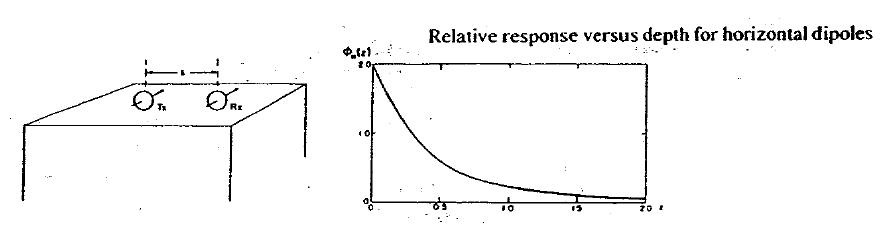
We therefore notice how two coil configurations couple differently with the ground and have different sensitivities with respect to the conductivity structure.

Cumulative Response Functions

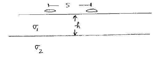
We often have a multi-layer earth (e.g. a thin resistive layer overlying a more conductive stratum, or vice versa) and we would like to estimate the thickness of the layer and the two conductivities. Cumulative response curves are useful for carrying out computations. Define

\[\begin{split}R_V (z) &= \int_{z}^{\infty} \phi_V (z) dz \\[0.8em] R_H (z) &= \int_{z}^{\infty} \phi_H (z) dz\end{split}\]

to be the relative contribution to the secondary magnetic field obtained from all of the material below a depth \(z\). The diagrams are plotted below:

A depth of investigation might be defined as that depth below which only 25% of the signal arises. According to this rule the depth of investigation for the vertical dipole is about 2.0 s while the depth for the horizontal dipole is only half that amount.

Multilayer Earth Structures

Under the assumption that \(s << \delta\) then the above formulae can be used to predict the apparent conductivity from a multilayered earth, or to used measured apparent conductivities to estimate the individual layer thickness and conductivities. For instance if we coplanar coils on the earth’s surface given below

The apparent conductivity would be

\[\begin{split}\sigma_a &= \int_{0}^{h} \sigma_1 \phi_V (z) dz + \int_{h}^{\infty} \sigma_2 \phi_V (z) dz \\[0.8em] &= \sigma_1 (1-R_V(h)) + \sigma_2 R_V(h)\end{split}\]

Either the curves shown previously or the following formulae are therefore useful:

\[\begin{split}\phi_V (z) &= \frac{4z}{(4z^2 + 1)^{3/2}} \\[0.8em] \phi_H (z) &= 2- \frac{4z}{(4z^2 + 1)^{1/2}} \\[0.8em] R_V &= \frac{1}{(4z^2 + 1)^{1/2} }\\[0.8em] R_H &= (4z^2 + 1)^{1/2} - 2z \\[0.8em]\end{split}\]

You can explore the response of a multilayered earth further using the layered earth response app.