Basic Principles

Here, we present the fundamental principles which govern ground penetrating radar (GPR) signals. As you will see, many of the basic fundamentals which are used to describe seismic methods can also be applied to GPR.

GPR Source

Fig. 90 Wavelet representing the pulse of EM waves within the GPR signal.

Fig. 91 GPR signals reflecting off a buried conductor.

As we mentioned earlier, the source of the GPR system sends a pulse of high-frequency electromagnetic waves (radiowaves) into the Earth (Fig. 90). Therefore, GPR equipment does not send a continuous signal into the Earth. The signal pulse contains a set of electromagnetic waves which oscillate near a particular frequency. And as these radiowaves propagate through the Earth, they are distorted due to the distribution of subsurface electromagnetic properties (\(\sigma , \; \mu\) and \(\varepsilon\)).

When radiowaves within the pulse come into contact with an interface (a boundary defined by an abrupt change in the Earth’s electromagnetic properties), portions of the incoming radiowaves can be reflected, transmitted and/or refracted (Fig. 91). The reflection, transmission and refraction of the radiowaves depends on the electromagnetic properties defining each side of the interface as well as the incident angle of the incoming radiowave signal.

For the purposes of GPR, the Earth may be thought of as a set of homogeneous regions separated by interfaces (Fig. 92). Using signals measured by the receivers, the goal of GPR is to define these interfaces and thus gain information about structures under the Earth’s surface; which can be naturally occurring or man-made.

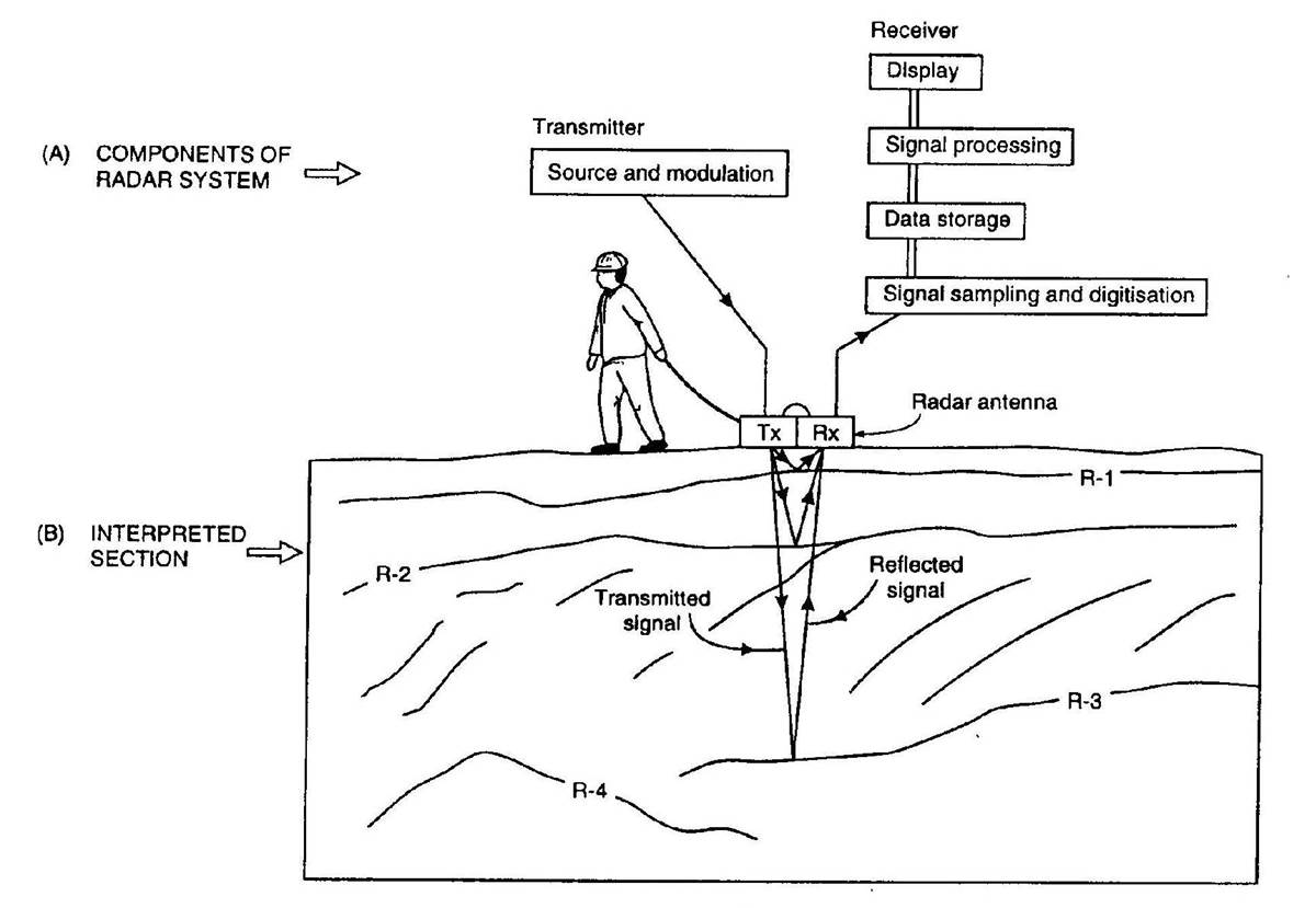
Fig. 92 Schematic of a zero-offset GPR setup.

Wave Velocity

Radiowaves propagate through different materials at different speeds. The velocity of the radiowaves depends on the physical properties of the medium. In general, the velocity of radiowaves through a homogeneous material is given by:

\[V = \sqrt{\frac{2}{\mu \varepsilon}} \Bigg [ \Bigg ( 1 + \bigg ( \frac{\sigma}{\omega \varepsilon} \bigg )^2 \, \Bigg )^{1/2} \; + 1 \; \Bigg ]^{-1/2}\]

This equation can be used to show that the radiowave velocity is largest in free-space (i.e. when \(\sigma = 0\), \(\mu = \mu_0\) and \(\varepsilon = \varepsilon_0\)). Therefore, electromagnetic waves in matter travel slower than the speed of light (c = 3.00 \(\times 10^8\) m/s).

GPR signals are characterized as being high-frequency. Thus in many cases (and for this course), it is safe to assume that \(\sigma \ll \omega \varepsilon\); especially if the Earth is resistive. This is known as the wave regime approximation. Using the approximation, the velocity of radiowaves can be simplified to:

\[V = \frac{1}{\sqrt{\mu \varepsilon}} = \frac{c}{\sqrt{\mu_r \varepsilon_r}}\]

where \(\mu_r\) is the relative permeability and \(\varepsilon_r\) is the relative permittivity. If the propagation material is non-magnetic, then \(\mu_r\) = 1 and the radiowave velocity simplifies to:

\[V = \frac{c}{\sqrt{\varepsilon_r}}\]

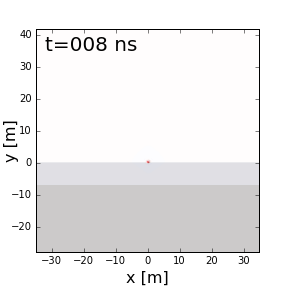
Fig. 93 GPR signal propagating through a layered Earth.

This expression is considered a good approximation when considering GPR signals. From the previous expression, we can see that radiowaves propagate more slowly in increasingly dielectric materials. A table showing the dielectric permittivity, conductivity and radiowave velocity for various materials can be found here . Notice that:

• Water saturation decreases the propagation velocity of sediments because they have high dielectric permittivities.

• Dry rocks and igneous rocks have the highest propagation velocity

Examine the GIF in Fig. 93. What medium has the higher velocity? What medium has the higher relative permittivity?

Attenuation

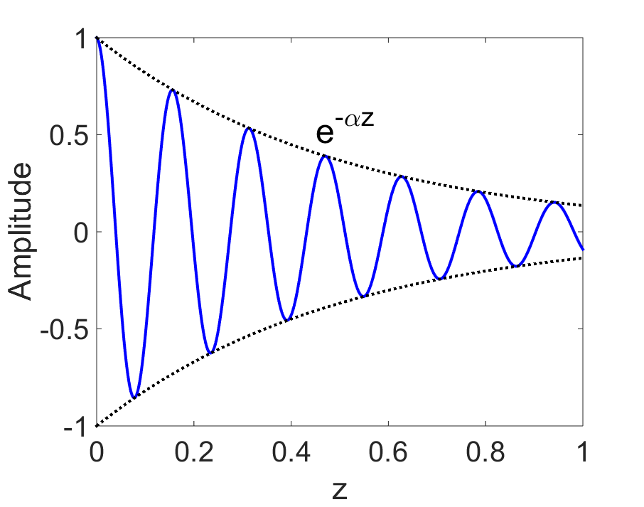
Fig. 94 Attenuation of electromagnetic waves.

Attenuation defines the continuous loss of amplitude a wave experiences as it propagates through a particular medium. The rate at which the amplitude decreases is referred as the attenuation constant (\(\alpha\)). For an electromagnetic wave that has traveled a distance \(z\), the attenuation constant is given by:

\[\frac{| \mathbf{A} |}{ | \mathbf{A_0} |} = e^{-\alpha z}\]

where \(\mathbf{A_0}\) is the initial amplitude of the wave and \(\mathbf{A}\) is the amplitude of the wave after it has travel distance \(z\). We can see that as \(z \rightarrow \infty\), the amplitude of the wave goes to zero. Additionally, for larger values of \(\alpha\), the wave attenuates more quickly.

The attenuation constant depends on the physical properties of the media. In general, the attenuation constant can be expressed as:

\[\begin{split}\alpha = \omega \sqrt{\frac{\mu \varepsilon}{2}} \Bigg [ \Bigg ( 1 + \bigg ( \frac{\sigma}{\omega \varepsilon} \bigg )^2 \Bigg )^{1/2} - \; 1 \; \Bigg ]^{1/2} \approx \begin{cases} \sqrt{\dfrac{\omega \mu \sigma}{2}} \; \; &\textrm{for} \; \; \omega \varepsilon \ll \sigma \\ \dfrac{\sigma}{2} \sqrt{\dfrac{\mu}{\varepsilon}} \; \; &\textrm{for} \; \; \sigma \ll \omega \varepsilon \end{cases}\end{split}\]

Once again, we see that the wave regime approximation (\(\sigma \ll \omega \varepsilon\)) for GPR provides a much simpler expression.

Skin Depth

Skin depth (\(\delta\)) defines the propagation distance at which the amplitude of an electromagnetic wave is reduced by a factor of \(1/e\); i.e. reduced to 37% of its original amplitude. By definition, the skin depth is just the reciprocal of the attenuation constant:

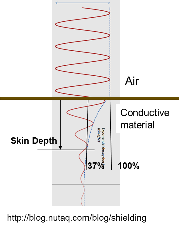
Fig. 95 Figure comparing the attenuation of radiowaves in air versus in a conductive medium.

\[\delta = \frac{1}{\alpha}\]

If we use the approximations found above and assume the Earth is non-magnetic (\(\mu_r = 1\)), the skin depth is given by:

\[\begin{split}\delta \approx \begin{cases} 503 \sqrt{\dfrac{1}{\sigma f}} \; \; &\textrm{for} \; \; \omega \varepsilon \ll \sigma \\ 0.0053 \dfrac{\sqrt{\varepsilon_r}}{\sigma} \; \; &\textrm{for} \; \; \sigma \ll \omega \varepsilon \end{cases}\end{split}\]

Where \(f\) is the frequency of the wave in Hz. We can see from the two previous expressions that:

• Generally, the skin depth is smaller if the frequency of the electromagnetic waves is higher.

• For the wave regime approximation (\(\sigma \ll \omega \varepsilon\)), skin depth reaches a limit which doesn’t depend on frequency.

• The skin depth is larger in materials with lower conductivities.

• The skin depth is larger is materials with higher dielectric permittivities.

An example of the attenuation of electromagnetic waves in air versus inside a conductive is shown on the right. We can see that in the air, the wave experienced little to no loss in amplitude as it propagates. In the conductive material however, the amplitude of the wave decreases noticeably as it propagates.

Reflection and Transmission of Radiowaves

Normal Incidence Reflection/Transmission

Fig. 96 Reflection of an incident wave with a reverse in polarity (\(\varepsilon_1 <\varepsilon_2\)). Link to source image .

When a radiowave reaches an interface, some of it is reflected and some of it is transmitted across the interface. This results in both a reflected and a transmitted wave.

The amplitude of the reflected wave proportional to that of the incident wave is defined by the reflection coefficient (\(R\)). For radiowaves, the reflection coefficient can be expressed as a function of the relative permittivities on each side of the interface. Assuming the radiowave arrives at an angle perpendicular to the interface, the reflection coefficient is given by:

\[R = \frac{\textrm{Reflected Amplitude}}{\textrm{Incident Amplitude}} = \frac{\sqrt{\varepsilon_1} - \sqrt{\varepsilon_2}}{\sqrt{\varepsilon_1} + \sqrt{\varepsilon_2}}\]

where \(\varepsilon_1\) is the relative permittivity of the medium carrying the incident and reflected waves. The transmission coefficient is given by:

\[T = \frac{\textrm{Transmitted Amplitude}}{\textrm{Incident Amplitude}} = \frac{2 \sqrt{\varepsilon_2}}{\sqrt{\varepsilon_1} + \sqrt{\varepsilon_2}}\]

The reflection coefficient can be either positive or negative and has values between \(-1 < R < 1\). The magnitude of \(R\) determines how much of the incident wave is reflected. It should be noted that:

• If \(\varepsilon_1\) and \(\varepsilon_2\) are similar, most of the incident wave is transmitted through the interface.

• If one of the relative permittivities across the interface is much smaller than the other, most of the incident wave is reflected. This can be a problem if you at attempting to gain information about structures below this interface.

The sign of the reflection coefficient determines whether the reflected wave experiences a reverse in polarity. As a result, we can use the polarity of reflected radiowaves to determine whether \(\varepsilon_1\) is greater than or less than \(\varepsilon_2\). This can be summarized as follows:

• If the returning signal (reflected wave) shows a reverse in polarity, \(R<0\) and thus \(\varepsilon_1 < \varepsilon_2\)

• If the returning signal (reflected wave) does not show a reverse in polarity, \(R>0\) and thus \(\varepsilon_1 > \varepsilon_2\)

Examine the GIF in Fig. 93. Look at the reflected wave as it returns to the surface. When it reaches the surface, is most of the wave reflected or transmitted? From this, are the relative permittivities of the air and the ground very different or similar?

Reflection at Conductive Object Boundaries

Many compact objects relevant to GPR applications (buried pipes, landmines, etc…) are highly conductive. For highly conductive objects, the reflection and transmission of radiowaves cannot be characterized by the dielectric permittivities. Instead, we must consider the electrical conductivity of the object.

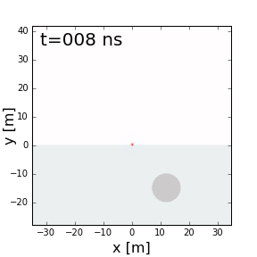
Fig. 97 GPR signals bouncing off of a conductive target.

From the general equation for propagation velocity, we see that as \(\sigma \rightarrow \infty\), the propagation velocity goes to zero. Thus radiowaves cannot propagate through extremely conductive objects. Because of this, when radiowaves reach the interface between the Earth and a highly conductive object, the wave is completely reflected. This occurs regardless of the incident angle.

Examine the GIF in Fig. 97. Can you see any of the wave being transmitted through the conductor?

Refraction of Radiowaves

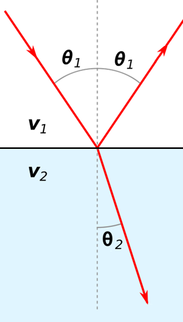
Fig. 98 Reflection and refraction of an incoming radiowave.

Refraction is used to describe the change in propagation direction of a wave due to a change in the propagation medium. When a radiowave reaches an interface, recall that some of it is reflected and some of it is transmitted accross the interface. The angles at which the incident wave is reflected and refracted are illustrated on the right.

The angle of the reflected portion depends directly on the angle of the incident wave. The angle of the refracted wave can be obtained by using Snell’s law (just like seismic waves):

\[\frac{\textrm{sin}\theta_1}{V_1} = \frac{\textrm{sin}\theta_2}{V_2}\]

For radiowaves in resistive and non-magnetic media, the propagation velocity is equal to \(V = c/ \! \sqrt{\varepsilon_r}\) (shown earlier). In this case, Snell’s law can be expressed as:

\[\sqrt{\varepsilon_1} \, \textrm{sin}\theta_1 = \sqrt{\varepsilon_2} \, \textrm{sin}\theta_2\]

where \(\varepsilon_1\) and \(\varepsilon_2\) are relative permittivities.

Remember that the GPR signal is a wavefront. If \(V_2 > V_1\), the wave wants to refract towards the horizontal. As a result, we expect the wavefront the ‘spread out’. Transversely, if \(V_2 < V_1\), the wave wants to refract towards the vertical and the wavefront should do the opposite. Go back to the GIF in Fig. 93 and examine the reflected wave that returns to the surface. Is the transmitted wave from the ground into the air spreading or contracting? What can you say about the velocities of both media?

Critical Refraction

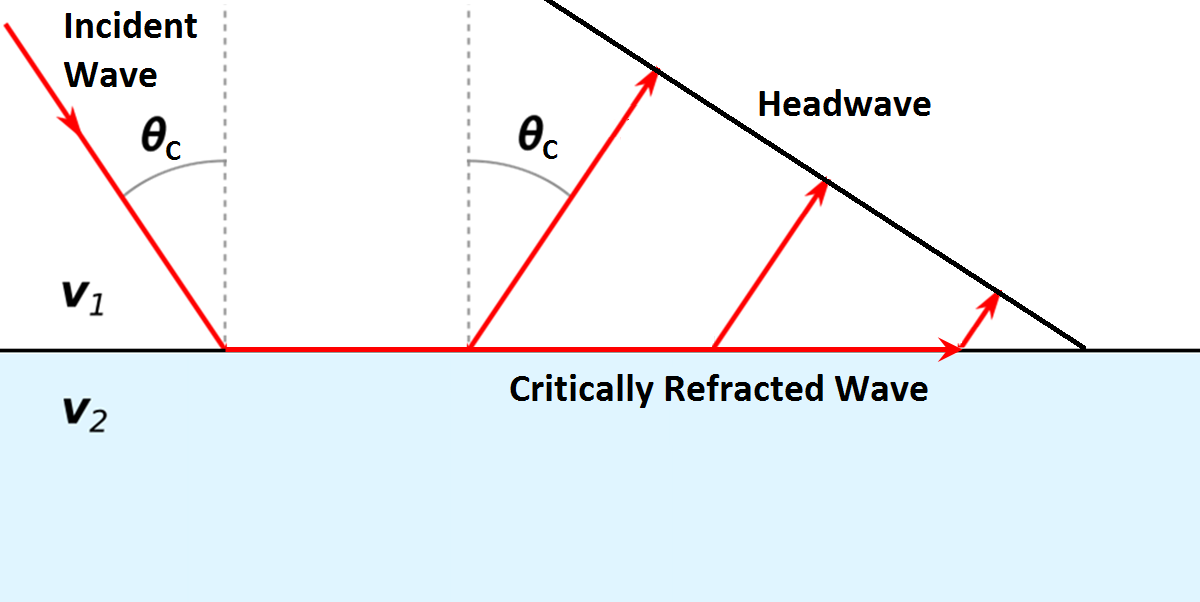
Fig. 99 Critical refraction at interface and the resulting head-wave.

Just like in refraction seismology, radiowaves can undergo critical refractions. This occurs when the incident angle \(\theta_1\) is such that the refracted wave propagates along the interface at velocity \(V_2\); ultimately leading to a head wave. The critical angle (\(\theta_c\)) is given by:

\[\textrm{sin} \theta_c = \frac{V_1}{V_2}\]

Once again, we can see that critical refraction only occurs when \(V_1 < V_2\). Additionally the propagation direction of the head wave is characterized by \(\theta_c\).

Scattering

Fig. 100 Scattering due to inhomogeneities.

Scattering is used to describe deviations in the paths of electromagnetic waves due to localized non-uniformities; which are less than 1/4 the wavelength of the radiowave signal. Scattering is problematic for GPR because it reduces the amplitudes of useful signals while increasing extraneous noise. Several sources of scattering are:

• Irregular surface shape of larger buried objects (below left).

• Rocky soils, which are a large contributor to the scattering of GPR signals (below right).

• Gas bubbles trapped in ice.

• Clutter made up of small buried objects

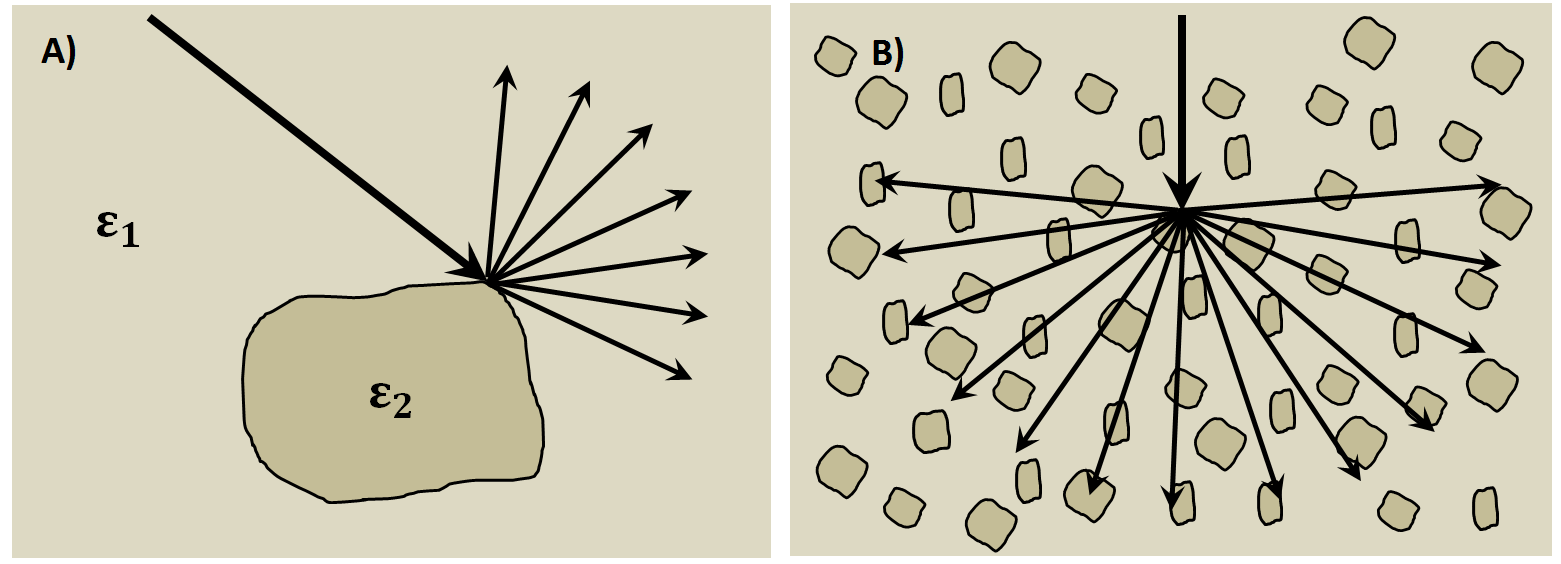
Fig. 101 Examples of scattering. A) Scattering from irregular surface texture. B) Scattering in rocky soils.

Wave Fronts and Ray Paths

Like in seismology, it is very important to understand the difference between wave-fronts and ray paths. One way to thing about it as follows:

• Wave-front: The physical location of the radiowave signal as it propagates through the Earth.

• Ray path: A particular path which a portion of the wave-front can take in order to reach a particular location.

Thus the wave-front represents the actual pulse of radiowaves, and the ray path is used to represent paths which signals can take to reach a receiver location. To see a simple example of the wavefront generated by radar source, see Fig. 93 of Fig. 97. To follow a ray path, choose a small sliver of the wavefront and follow it as it reflects, refracts and propagates. If at any time this portion of the wavefron reaches the receiver, it is a ray path which is measured.

Geometric Spreading

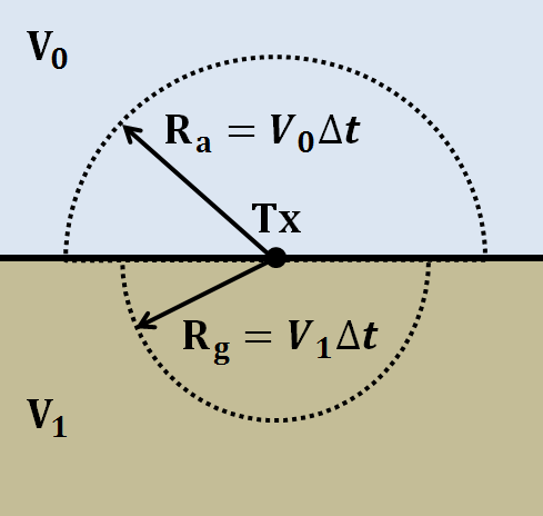
Fig. 102 Wave-front at time \(\Delta t\). Shows geometric spreading for radiowaves in the ground and in the air.

We have seen how radiowave signals lose their amplitude through attenuation. They also lose amplitude due to geometric spreading. This makes sense given that the energy of the wave-front is now spread over an increasingly larger area. For geometric spreading, the loss in amplitude of the radiowaves is represented by:

\[\frac{| \mathbf{A} |}{ | \mathbf{A_0} |} \propto \frac{1}{R}\]

where \(\mathbf{A_0}\) is the amplitude of the waves as their leave the source and \(\mathbf{A}\) is the amplitude of the waves after they have traveled distance \(R\). As we can see from the figure, the rate of geometric spreading loss is higher in the air than it is in the ground. This is due to the fact that radiowaves propagate faster in the air than they do in the ground. Examine Fig. 93. Can you see spherical spreading? In what medium is spherical spreading happening more quickly?

Example: Signal Paths for a 2-Layer Earth

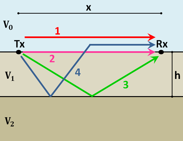
Fig. 103 Radiowaves signals measured by a receiver for a 2-layer Earth.

Now that we understand the background theory, let’s put it all together. At \(t\) = 0 s, the source (Tx) generates a pulse of radio waves. As we can see on the right, there are many paths in which radiowaves can take in order to reach the receiver (Rx). The propagation velocities, reflections and refractions can all be explained using the equations found above. On the right, we have an example of a radargram, which shows the returning signal at increasing distances \(x\) from the source. Let us now try and explain the nature of each ray path.

Path 1: Direct Air Wave

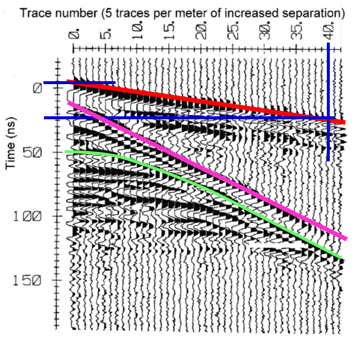
Fig. 104 Radargram for a 2-layer Earth.

This was travels through the air in a direct line from the transmitter to the receiver. Recall that in the air, radiowaves propagate roughly at the speed of light (\(c = 3.00 \times 10^8\) m/s). As a result, the direct air wave is always the first signal measured by the receiver. The time it takes this wave to reach the receiver is given by:

\[t_{air} = \frac{x}{c}\]

The direct wave is shown in red on the radargram. According to the above equation, the velocity of the air wave is 1 divided by the slope of this line.

Path 2: Direct Ground Wave

This wave travels along the surface interface at velocity \(V_1\). Like the air wave, the ground wave also takes a direct path. Because \(V_1 < c\), the ground wave arrives later than the air wave. The time it takes for the ground wave to reach the receiver is given by:

\[t_{ground} = \frac{x}{V_1}\]

The direct ground wave is shown in pink. Like the air wave, the direct ground wave velocity can also be obtained from the slope of the line.

Path 3: Reflected Wave

The reflected wave travels through medium 1 at velocity \(V_1\). Because it takes a longer path than the direct ground wave, it arrives later. The time it takes for the reflected wave to reach the receiver is given by:

\[t_{ref} = \frac{\sqrt{x^2 + 4h^2}}{V_1}\]

The reflected wave is shown in green. Unlike direct waves, the arrival time for the reflected wave is hyperbolic, which makes it distinguishable from other signals. After sufficient distances (\(h \ll x\)), the previous equation becomes approximately linear. This portion of the curve can be used to estimate the velocity of the top-most layer. Notice how the slope of the direct ground wave and reflected wave are parallel.

Path 4: Critically Refracted at Surface

This ray path is denoted in blue. Because \(V_1 < V_0\), reflected waves are critically refracted at the surface. While this wave propagates along the surface interface, it will have velocity a velocity roughly the speed of light. In general, the time it takes for this wave to reach the receiver is given by:

\[t_c = \frac{x}{c} + \textrm{Constant}\]

Notice that the arrival time for the critically refracted wave is linear. In this radargram example, we cannot easily see the critically refracted wave. However, it does not mean that it does not exist.